
Partial Autocorrelation Function
On this page
Purpose
The Partial Autocorrelation Function (PACF) measures the correlation between a series and itself k periods earlier after the effect of the shorter lags 1 … k − 1 has been taken out. Where the ordinary autocorrelation (ACF) shows every lag as related when there is a strong carry-over, the PACF shows which lags carry information of their own. Use it with the ACF to choose the autoregressive (AR) order of an ARIMA model, and on model residuals to check for a pattern left over.
Key Capabilities
- Partial autocorrelation at every lag from 1 up to the number of lags you choose, or a default based on the series length.
- Correlogram (bar chart) with dashed significance limits at about ±2/√n.
- T statistic for each lag in a table next to the PACF values.
- Works on any numeric column in time order; the series must have no gaps.
Statistical Methods
The tool first computes the sample autocorrelations r₁ … rₘ, then the partial autocorrelations φₖₖ by the Durbin-Levinson recursion: φₖₖ = (rₖ − Σⱼ<ₖ φₖ₋₁,ⱼ·rₖ₋ⱼ) / (1 − Σⱼ<ₖ φₖ₋₁,ⱼ·rⱼ), with φₖ,ⱼ = φₖ₋₁,ⱼ − φₖₖ·φₖ₋₁,ₖ₋ⱼ. φₖₖ equals the last coefficient of an AR(k) model fitted to the autocorrelations, so it is the part of the lag k correlation not explained by lags 1 to k − 1.
For a random series the PACF at each lag has a standard error of about 1/√n. The T column is φₖₖ·√n and the significance limits are ± t₀.₉₇₅,ₙ₋₁ / √n, the same at every lag. A bar outside the limits is unlikely to be chance at the 5% level. When Number of lags is blank, the tool uses n/4 lags (√n + 45 when n > 240), and never more than n − 1.
How to read the pattern: a PACF that cuts off after lag p (large bars at lags 1 … p, small after) while the ACF decays gradually points to an AR(p) model. Spikes at and around the seasonal lag (12 for monthly data) point to a seasonal term. A PACF that decays gradually while the ACF cuts off points to a moving average model instead.
Input Fields & Options
Field | Description |
Variable | Required. The numeric column holding the series, in time order. |
Number of lags | Optional, 1 to 1000. The highest lag shown. Blank uses n/4 (√n + 45 when n > 240). For seasonal data choose at least two full seasons, e.g. 24 for monthly data. |
Title | Title shown on the graph. Default Partial Autocorrelation Function. |
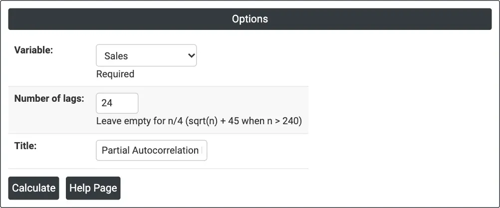
Figure 1 — Partial autocorrelation of monthly Sales for 24 lags.
Output Descriptions
- Partial Autocorrelation Function (graph) — a bar for each lag with the dashed significance limits.
- Partial Autocorrelation Function: <variable> (table) — Lag, PACF and T for each lag.
- PDF export via Download.
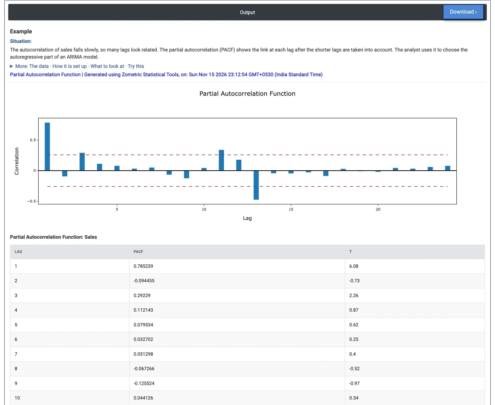
Figure 2 — PACF of monthly sales: one large spike at lag 1 (0.79) and spikes at lags 11 and 13 around the yearly season.
Worked Example
A consumer electronics distributor has 60 months of unit sales, January 2020 to December 2024. The autocorrelations fall slowly, so many lags look related. To choose the AR part of an ARIMA model, the sales analyst runs the PACF with Variable = Sales and Number of lags = 24.
With n = 60 the significance limits are ±0.26. Lag 1 has a single large spike of 0.79 (T 6.08): last month's sales carry most of the information about this month, the sign of an AR(1) term. Lag 2 is small (−0.09). Lag 3 is just outside the limits at 0.29 (T 2.26), a weak effect that is easy to over-read. Lags 11 and 13 stand out at 0.34 (T 2.63) and −0.48 (T −3.69); spikes around lag 12 show the yearly season, which a seasonal difference or seasonal term handles better than extra AR lags.
The decision is an AR(1) term together with a seasonal part, which is the model used on the ARIMA page (AR 1 with a 12-month seasonal difference and a seasonal MA term). Advertising Spend shows the same mix: spikes at lags 1 (0.62), 11, 12 and 13 (−0.47), month-to-month carry-over plus the yearly calendar.