
Poisson Regression
On this page
Purpose
Poisson Regression relates a count response, such as defects per shift, breakdowns per month or flaws per panel, to continuous and categorical predictors. Use it instead of ordinary regression when the response is a count of events in a fixed amount of time, area or product: the counts cannot be negative and their spread grows with their mean, which least squares does not allow for.
Key Capabilities
- Continuous and categorical predictors, with interactions and squared terms from the term list.
- Log (default), square root or identity link.
- Stepwise, forward selection or backward elimination of terms, with terms forced into every model.
- Coefficients with confidence intervals and VIF, regression equations for each level of a categorical predictor, model summary and goodness-of-fit tests.
- Analysis of deviance by Wald or likelihood-ratio tests (adjusted or sequential).
- Unusual observations, residual plots, main effects and interaction plots, contour and surface plots of fitted counts.
- Prediction at settings you enter and a response optimizer.
Statistical Methods
The response is assumed to follow a Poisson distribution with mean μ that depends on the predictors through the link: with the log link, ln μ = b₀ + b₁x₁ + … , so each coefficient multiplies the expected count by exp(b) per unit of its predictor. The model is a generalised linear model fitted by maximum likelihood (iteratively reweighted least squares). Categorical predictors use (1, 0) coding against a reference level, by default the first level in sort order. Rows with a missing value are dropped; a frequency column repeats rows and a weights column gives variance weights.
The coefficient table gives Wald z-values (Coef / SE Coef) and confidence intervals. The analysis of deviance tests each term: by default with a Wald chi-square (z² for a continuous term, a joint test for the dummy columns of a categorical term); with the LR test, by the change in deviance when the term is dropped from the full model (adjusted, Type III) or added in order (sequential, Type I). Deviance R-Sq = 1 − residual deviance / null deviance.
Goodness-of-fit tests compare the deviance and the Pearson chi-square with a chi-square distribution on the error degrees of freedom. A small p-value, or a Mean (deviance / DF) well above 1, means the counts vary more than a Poisson model allows (overdispersion), and the p-values for the terms are then too small. Observations with a standardised residual beyond ±2 are flagged R, and those with leverage above 3p/n are flagged X.
Input Fields & Options
Field | Description |
Response | Column of counts. Required. |
Continuous Predictors / Categorical Predictor | Numeric and text (or coded) predictor columns; at least one. Ctrl or Command + click to select several. |
Model terms (optional) | Term list: tick terms, or use Add all, Interactions and Powers up to the order chosen in Terms through order (2 or 3). Untick In model to remove a linear term while keeping its interactions. |
Reference level (optional) | For categorical predictors, “Predictor Level”, comma-separated. Default: first level in sort order. |
Stepwise method | None (default), Stepwise, Forward selection or Backward elimination; with Alpha to enter and Alpha to remove (0.15), hierarchy rules, Terms in every model (E), Initial model terms (I) and Model selection details. |
Frequency (optional) / Weights (optional) | Columns of row frequencies and of weights. |
Link function | Log (default), Square root or Identity. |
Confidence level / Type of confidence interval | Default 95, Two-sided; or Lower bound or Upper bound. |
Fits and diagnostics for all observations | Lists fit and residual for every row, not only unusual ones. |
Test for ANOVA table / Type of deviance (LR test only) | Wald test (default) or LR test; for LR, Adjusted (Type III, default) or Sequential (Type I). |
Residuals for diagnostics/plots | Deviance (default) or Pearson. |
Histogram of residuals / Normal probability plot of residuals / Residuals versus fits / Residuals versus order / Four in one / Residuals versus the variables | Residual plots. |
Main effects plot / Interaction plot | Fitted count against each predictor, the others held at their mean or reference level. |
Contour plot / Surface plot / Overlaid contour plot of fitted values | Need X1 and X2 axis variables; the overlaid contour plot also needs Response low and Response high. |
Prediction / Response Optimizer | Add a panel to predict the mean count (with SE and confidence interval) at settings you enter, or to search for settings that meet a count goal. |
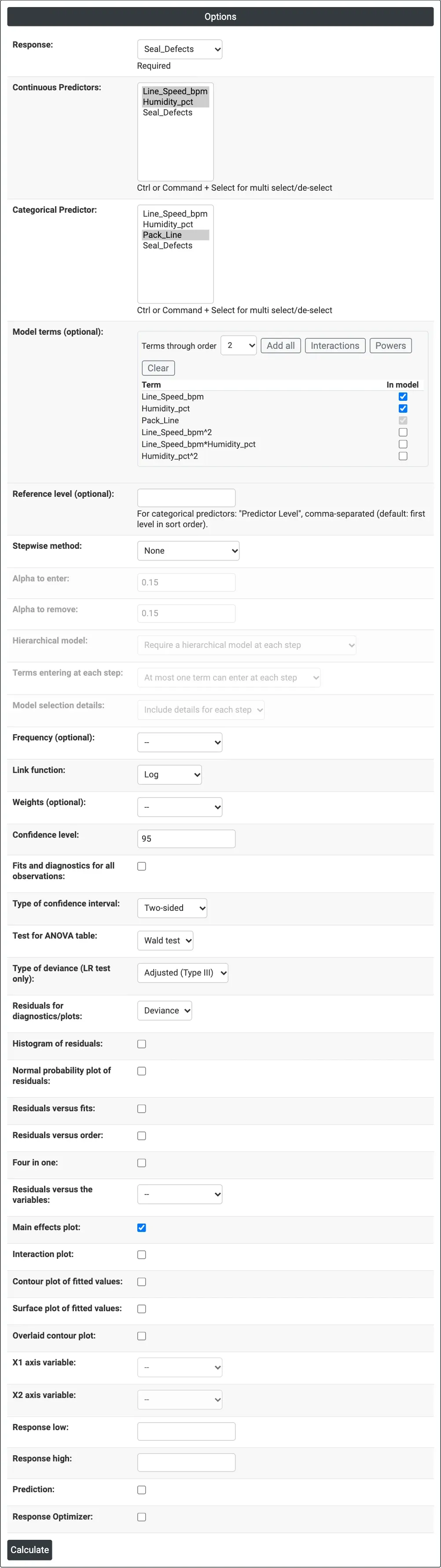
Figure 1 — Options for the bag seal example: Seal_Defects as the response, line speed and humidity as continuous predictors, packing line as a categorical predictor, main effects plot ticked.
Output Descriptions
- Method — link function, categorical coding and rows used.
- Response Information — N, mean, standard deviation, minimum and maximum of the counts.
- Coefficients — Coef, SE Coef, Z-Value, P-Value, confidence limits and VIF.
- Regression Equation — the linear predictor Y' (ln of the expected count with the log link) for each level of the categorical predictors.
- Model Summary — deviance R-Sq, Adj R-Sq, AIC, AICc and BIC.
- Goodness-of-Fit Tests — deviance and Pearson chi-square tests.
- Fits and Diagnostics for Unusual Observations.
- Analysis of Deviance — chi-square and p-value for the regression and each term.
- Stepwise selection table, residual, factorial, contour and surface plots, prediction and optimizer panels when selected.
- PDF export via Download.
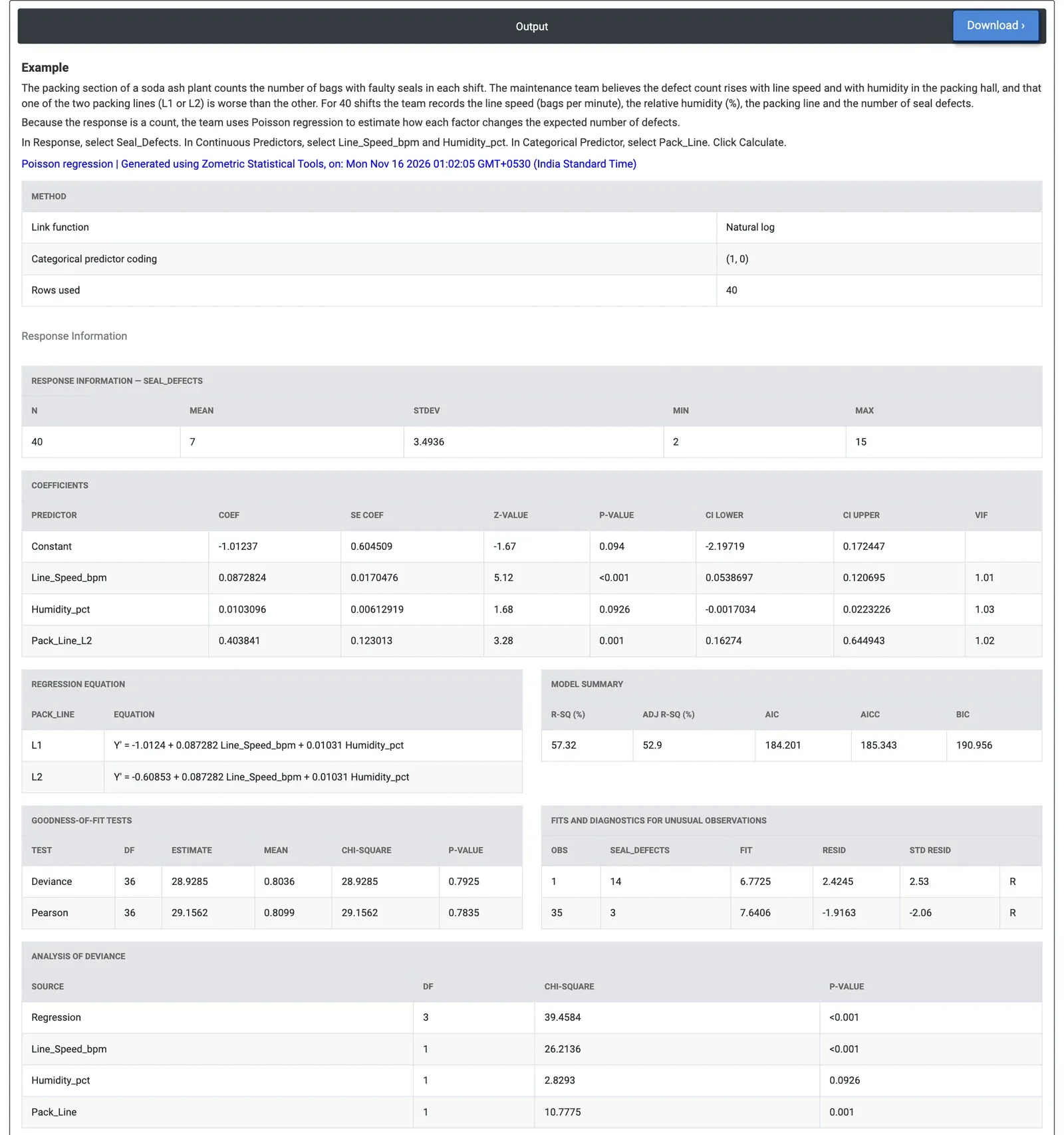
Figure 2 — Poisson regression of seal defects per shift: line speed (p < 0.001) and packing line (p = 0.001) matter, humidity does not at the 5% level (p = 0.0926).
Worked Example
The packing section of a soda ash plant counts the bags with faulty seals in each shift. For 40 shifts the team records the line speed (bags per minute), the humidity in the packing hall (%), the packing line (L1 or L2) and the number of seal defects (2 to 15, mean 7). They select Seal_Defects as the response, line speed and humidity as continuous predictors and Pack_Line as the categorical predictor, and keep the log link.
Line speed has the strongest effect (Wald chi-square 26.21, p < 0.001): its coefficient 0.0873 means each extra bag per minute multiplies the expected defects by exp(0.0873) = 1.09, and 5 bags per minute faster by about 1.55. Line L2 has coefficient 0.404 (p = 0.001), so at the same speed and humidity it makes about 1.50 times as many seal defects as L1. Humidity points the same way (about 11% more defects per 10% RH) but is not significant at the 5% level (p = 0.0926).
The model fits the counts: deviance chi-square 28.93 on 36 DF (p = 0.7925) and Pearson 29.16 (p = 0.7835), with Mean below 1, so there is no sign of overdispersion. Two shifts are flagged: shift 1 with 14 defects against a fit of 6.8, and shift 35 with 3 against 7.6. The team looks first at the seal jaws on L2 and at the speed set point, and keeps collecting humidity data before deciding on dehumidification.