
Power and Sample Size for 1 Proportion
On this page
Purpose
Power and Sample Size for 1 Proportion plans a test of a single proportion before you collect the data, for example the defective rate of a process, the share of first-pass yield or the proportion of late deliveries, compared with a target or historical value. Enter any two of sample size, alternative proportion and power, and the tool solves for the third: how many items to inspect, what chance a planned sample gives of detecting the change, or the smallest change a given sample can detect. Use it before a 1 Proportion test.
Key Capabilities
- Solves for sample size, power or alternative proportion: leave blank the one you want.
- Several values at once, e.g. alternative proportions “0.02 0.03” and power values “0.8 0.9”, give one row for each combination.
- Two-sided (Proportion ≠ hypothesized proportion) or one-sided (less than, greater than) alternatives, at the confidence level you choose.
- When solving for sample size, reports the whole number of items and the actual power it gives.
- Power curve of power against sample size for each alternative proportion, with the solved points marked.
Statistical Methods
The tool uses the normal approximation to the binomial distribution (the exact binomial method is not offered). The significance level is α = 1 − confidence level / 100. Let p₀ be the hypothesized proportion, p₁ the alternative proportion and z the critical value: z₁₋α/₂ for the two-sided alternative and z₁₋α for a one-sided one.
For the “greater than” alternative let Δ = p₁ − p₀, for “less than” Δ = p₀ − p₁, and for the two-sided alternative Δ = |p₁ − p₀|. Power at sample size n is Φ((Δ·√n − z·√(p₀(1 − p₀))) / √(p₁(1 − p₁))), where Φ is the standard normal distribution function. The sample size for a target power is n = ((z·√(p₀(1 − p₀)) + z_β·√(p₁(1 − p₁))) / Δ)², with z_β the normal quantile of the target power; n is rounded up to the next whole number and the power at that n is reported as the actual power. When solving for the alternative proportion, the tool searches below p₀ for the “less than” alternative and above p₀ otherwise (so a two-sided run reports the value above p₀).
A one-sided test only has power when the alternative proportion lies on the side the alternative names: with Proportion < hypothesized proportion, an alternative proportion above p₀ gives a power near 0, and solving for sample size from it returns an error message. Proportions near 0 or 1 make the normal approximation less accurate; with very small defect rates treat the answer as a guide. Power rises with sample size and with the gap, and falls as the confidence level rises.
Input Fields & Options
Field | Description |
Sample sizes | Number of items. Space or comma-separated, e.g. “50 100 150”. Leave blank to solve for sample size. |
Hypothesized proportion | Required. The target, claimed or historical proportion p₀, between 0 and 1. |
Alternative proportion(s) | Space or comma-separated, e.g. “0.5 0.6”. The proportion(s) you want to detect. Leave blank to solve for it. |
Power values | Space or comma-separated, e.g. “0.8 0.9”. Leave blank to solve for power. |
Confidence level | Default 95 (α = 0.05); 75 to 100. |
Alternative hypothesis | Proportion ≠ hypothesized proportion (default), Proportion < hypothesized proportion or Proportion > hypothesized proportion. |
Power curve | Ticked by default: draws power against sample size. |
Title | Title shown on the output and the power curve. |
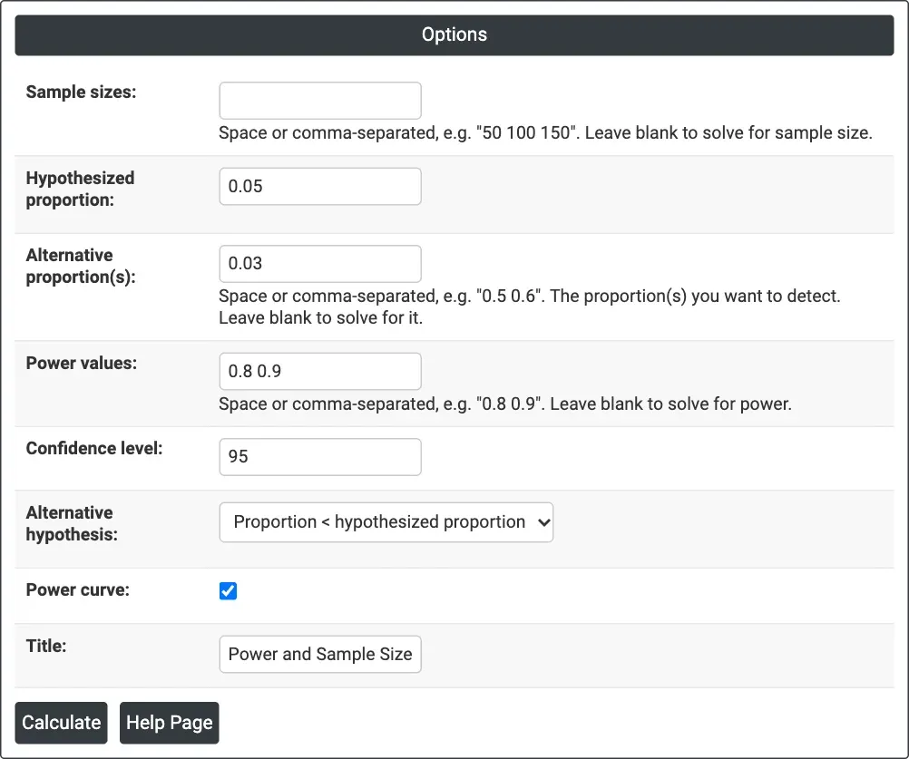
Figure 1 — Solving for sample size: Hypothesized proportion = 0.05, Alternative proportion(s) = 0.03, Power values = 0.8 0.9, one-sided (Proportion < hypothesized proportion) at 95% confidence.
Output Descriptions
- Settings — what was solved for, the hypothesized proportion, the confidence level and the alternative hypothesis.
- Results — one row per combination: alternative proportion, sample size, and target and actual power when solving for sample size, or power when solving for power, or the alternative proportion when solving for it.
- Power Curve — power against sample size for each alternative proportion, with the calculated points marked.
- PDF export via Download.
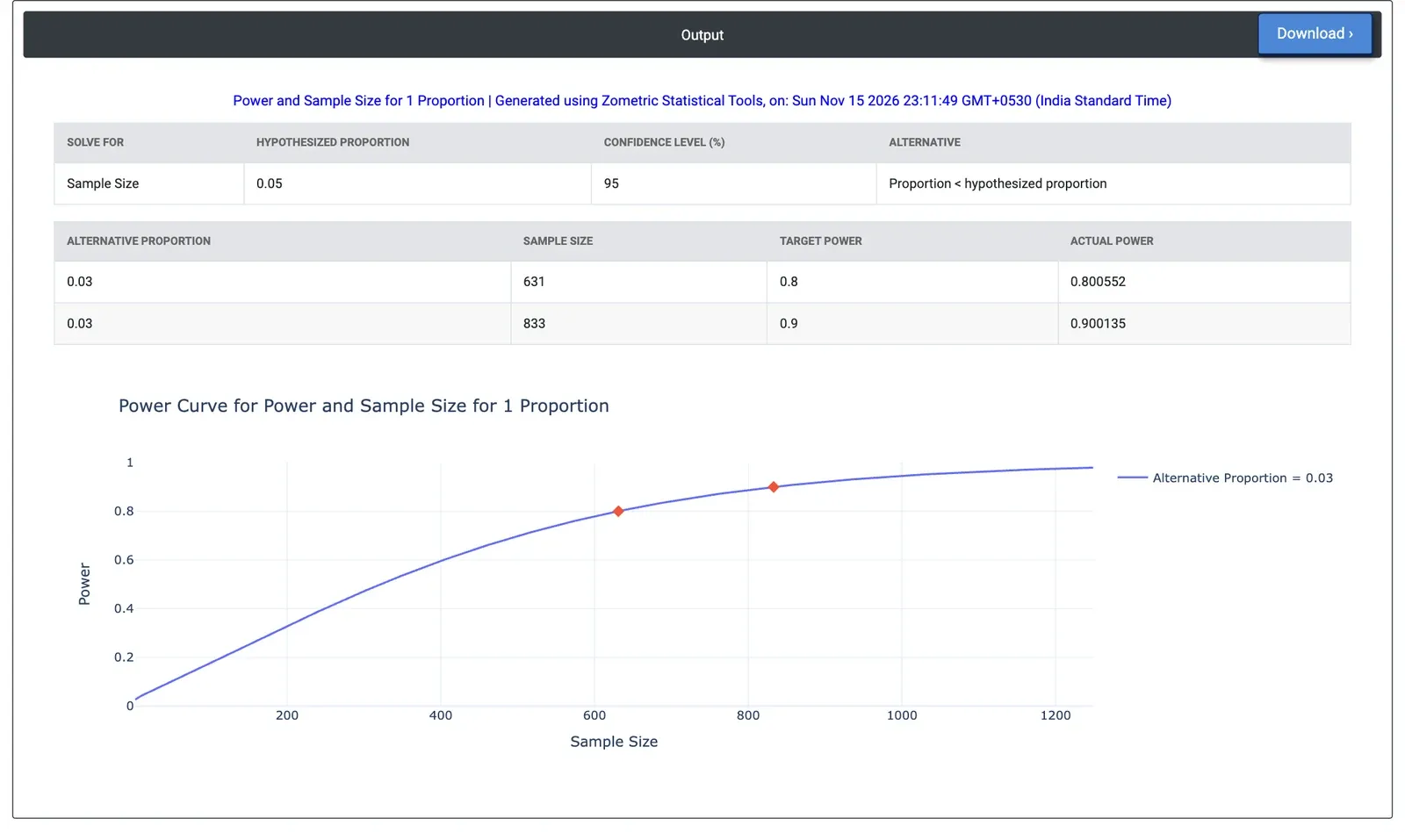
Figure 2 — Results for the example: 631 parts for 80% power and 833 for 90% power to detect a drop from 5% to 3% defective.
Worked Example
A moulding cell has run at 5% defective for the past year. A process change is expected to bring this down to 3%, and the team wants a trial run large enough to show the drop with a 1 Proportion test. Only a decrease matters, so they choose the one-sided alternative Proportion < hypothesized proportion. They leave Sample sizes blank and enter Hypothesized proportion = 0.05, Alternative proportion(s) = 0.03 and Power values = 0.8 0.9, at 95% confidence.
The tool needs 631 parts for 80% power (actual power 0.801) and 833 parts for 90% power (actual power 0.900). Small defect rates need large samples: with a trial of only 300 parts the power is 0.472, so the trial would miss a real drop to 3% about half the time. With 300 parts and 80% power, the smallest drop the test can reliably show is to about 2.2% (alternative proportion 0.0222). A two-sided test would need 815 parts for 80% power, and a larger expected improvement, to 2%, needs only 253 parts for 80% power with the one-sided test.