
Power and Sample Size for 1-Sample Equivalence Test
On this page
Purpose
Power and Sample Size for 1-Sample Equivalence Test plans a study that has to show a process mean is close enough to a target, rather than different from it. You set an equivalence window (lower and upper limits on mean − target) and the tool tells you how many measurements are needed to prove the mean lies inside it, what power a planned sample gives, or how far from the target the true mean can be for a given sample and power. Enter any two of sample size, difference and power, and the tool solves for the third. Use it before a 1-Sample Equivalence Test, for example when validating a new filling head, gauge or recipe against a nominal value.
Key Capabilities
- Solves for sample size, power or difference: leave blank the one you want.
- Several values at once, e.g. differences “0 0.5 1” and power values “0.8 0.9”, give one row for each combination.
- Any equivalence window: symmetric (−2 to 2) or not (−1 to 3).
- Exact power for the two one-sided tests (TOST) procedure, using the t distribution rather than a normal approximation.
- Power curve of power against sample size for each difference, with the solved points marked.
Statistical Methods
The equivalence test uses two one-sided t-tests (TOST). With n measurements, standard deviation σ, standard error SE = σ/√n and n − 1 degrees of freedom, equivalence is claimed when the mean minus the target is shown to be above the lower limit L and below the upper limit U, each at significance level α (the Significance level (alpha) field, default 0.05; it is not split in two).
Power is the probability that both one-sided tests succeed when the true difference (mean − target) is δ. The tool computes it exactly: for a given sample standard deviation the chance of success is a difference of two normal probabilities, Φ(−t·s/σ − (δ − U)/SE) − Φ(t·s/σ − (δ − L)/SE) with t = t₁₋α,n−1, and this is averaged over the chi-square distribution of the sample variance by numerical integration. For sample size, the n that reaches the target power is found and rounded up, and the power at that n is reported as the actual power. When solving for the difference, the tool searches between the midpoint of the limits and the upper limit, because power is highest when the true difference sits at the midpoint and falls towards either limit.
The difference to detect must lie strictly between the limits: a true mean at or beyond a limit can never be shown equivalent. Power rises with the sample size and the width of the window, and falls as σ grows or the true difference moves towards a limit.
Input Fields & Options
Field | Description |
Sample sizes | Space or comma-separated, e.g. “20 30 40”. Leave blank to solve for sample size. |
Difference(s) to detect | Space or comma-separated, e.g. “0.5 0.7”. The true difference (mean − target) you expect; must lie strictly between the lower and upper limits. Leave blank to solve for it (searches between the midpoint of the limits and the upper limit). |
Power values | Space or comma-separated, e.g. “0.8 0.9”. Leave blank to solve for power. |
Lower equivalence limit / Upper equivalence limit | Required. The smallest and largest acceptable difference from the target, in measurement units; the lower limit must be less than the upper limit. |
Standard deviation | Required. Assumed or historical standard deviation of the measurements. |
Significance level (alpha) | Default 0.05. Applied to each of the two one-sided tests. |
Power curve | Ticked by default: draws power against sample size. |
Title | Title shown on the output and the power curve. |
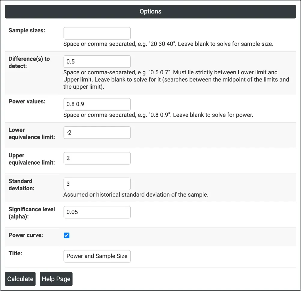
Figure 1 — Solving for sample size: Difference(s) to detect = 0.5, Power values = 0.8 0.9, limits −2 and 2, Standard deviation = 3, alpha = 0.05.
Output Descriptions
- Settings — what was solved for, the lower and upper equivalence limits, the standard deviation and the significance level.
- Results — one row per combination: difference, sample size, and target and actual power when solving for sample size, or power when solving for power, or difference when solving for difference.
- Power Curve — power against sample size for each difference, with the calculated points marked.
- PDF export via Download.
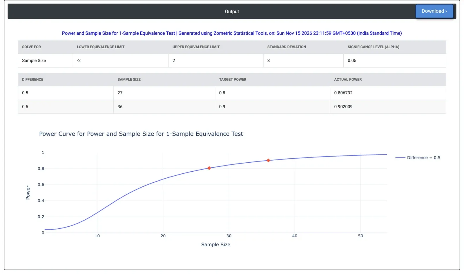
Figure 2 — Results for the example: 27 fills for 80% power and 36 for 90% power when the true offset is 0.5 g inside a ±2 g window.
Worked Example
A packaging line fits a new filling head and must show that its mean fill is within ±2 g of the 500 g target before release. Historical data put the fill standard deviation at 3 g, and the engineers expect the new head to run up to 0.5 g off target. They leave Sample sizes blank and enter Difference(s) to detect = 0.5, Power values = 0.8 0.9, Lower equivalence limit = −2, Upper equivalence limit = 2 and Standard deviation = 3, with alpha = 0.05.
The tool needs 27 fills for 80% power (actual power 0.807) and 36 fills for 90% power (actual power 0.902). With only 20 fills the power is 0.669, a one-in-three chance that a head which really is acceptable fails the equivalence test. The offset matters: a head running exactly on target needs 21 fills for 80% power, while one running 1 g off target needs 58. If the team is unsure of the offset, planning for the larger value protects the study.