
Power and Sample Size for 1-Sample t
On this page
Purpose
Power and Sample Size for 1-Sample t plans a test of one mean against a target or nominal value before you collect the data: how many measurements are needed to detect a shift that matters, what chance (power) a planned sample gives of detecting it, or the smallest shift a given sample can detect. Enter any two of sample size, difference and power, and the tool solves for the third. Use it before a 1-sample t-test, for example to check whether a machine is centred on nominal or whether a material meets a specified mean.
Key Capabilities
- Solves for sample size, power or difference: leave blank the one you want.
- Several values at once, e.g. differences “0.01 0.02” and power values “0.8 0.9”, give one row for each combination.
- Two-sided (Mean ≠ hypothesized mean) or one-sided (Mean < hypothesized mean, Mean > hypothesized mean) alternatives, at the confidence level you choose.
- When solving for sample size, reports the whole number of measurements and the actual power it gives.
- Power curve of power against sample size for each difference, with the solved points marked.
Statistical Methods
The calculation assumes the measurements come from a normal population whose standard deviation σ is estimated from the sample, as in the 1-sample t-test. The significance level is α = 1 − confidence level / 100, and the standardised difference is d = difference / σ, where the difference is the true mean minus the hypothesized mean.
Power is the probability that the t-test rejects the null hypothesis when the true mean differs from the hypothesized mean by the difference entered. It is computed from the noncentral t distribution with n − 1 degrees of freedom and noncentrality parameter δ = d·√n: for a two-sided test, power = P(T > t₁₋α/₂) + P(T < −t₁₋α/₂), where T follows that noncentral t; for a one-sided test only the tail on the side of the alternative counts. For sample size, the n that gives the target power is found and rounded up to the next whole number, and the power at that n is reported as the actual power. For difference, the smallest difference that reaches the target power with the given n is found.
Power rises with the sample size and the size of the difference, and falls as σ grows or the confidence level rises. A one-sided test needs fewer measurements for the same power but only detects a shift in the stated direction: with Mean > hypothesized mean, a negative difference gives a power near 0, and solving for sample size from it returns an error message. For the two-sided test only the size of the difference matters. Solving for difference with Mean < hypothesized mean returns a negative difference.
Input Fields & Options
Field | Description |
Sample sizes | Space or comma-separated, e.g. “10 20 30”. Leave blank to solve for sample size. |
Differences | Space or comma-separated, e.g. “1 2 3”. The difference from the hypothesized mean you want to detect, in measurement units. Leave blank to solve for difference. |
Power values | Space or comma-separated, e.g. “0.8 0.9”. Leave blank to solve for power. |
Standard deviation | Required. Assumed or historical standard deviation of the population, e.g. from past data or a pilot run. |
Confidence level | Default 95 (α = 0.05); 75 to 100. |
Alternative hypothesis | Mean ≠ hypothesized mean (default), Mean < hypothesized mean or Mean > hypothesized mean. |
Power curve | Ticked by default: draws power against sample size. |
Title | Title shown on the output and the power curve. |
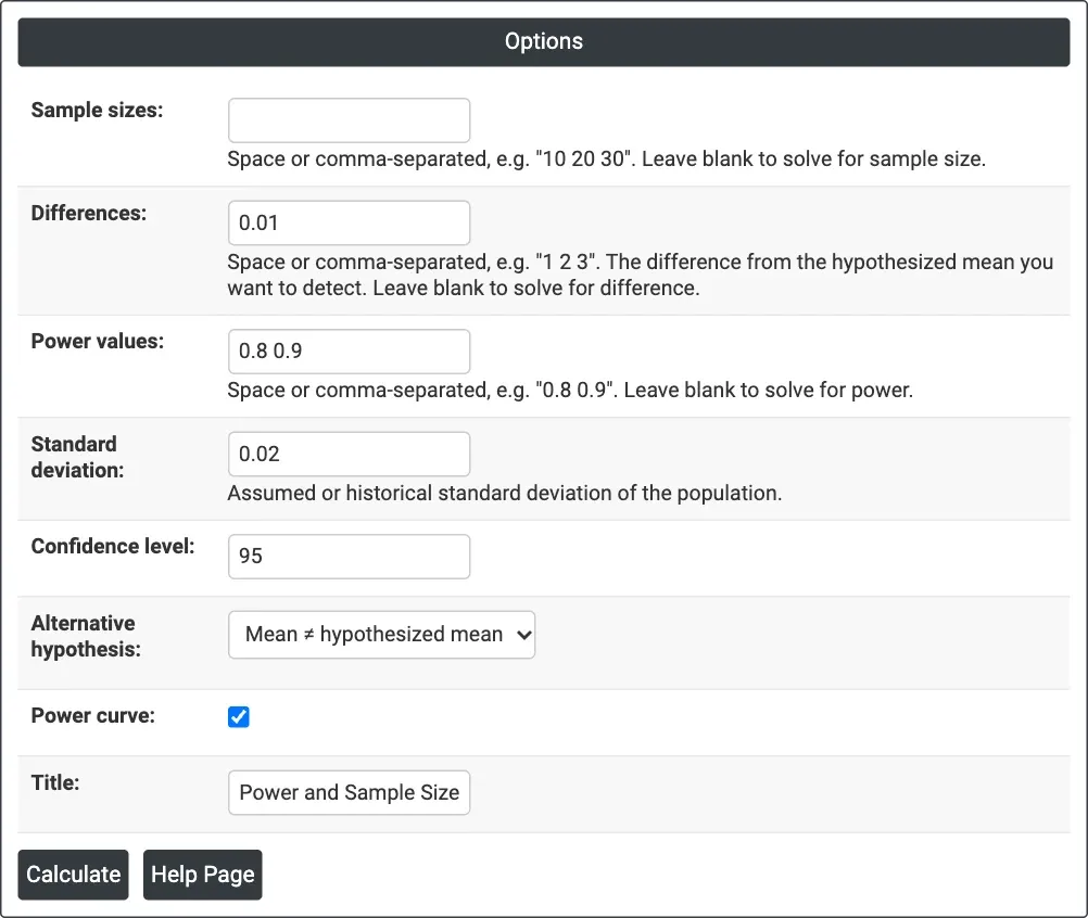
Figure 1 — Solving for sample size: Differences = 0.01, Power values = 0.8 0.9, Standard deviation = 0.02, two-sided at 95% confidence.
Output Descriptions
- Settings — what was solved for, the standard deviation, the confidence level and the alternative hypothesis.
- Results — one row per combination: difference, sample size, and target and actual power when solving for sample size, or power when solving for power, or difference when solving for difference.
- Power Curve — power against sample size for each difference, with the calculated points marked.
- PDF export via Download.
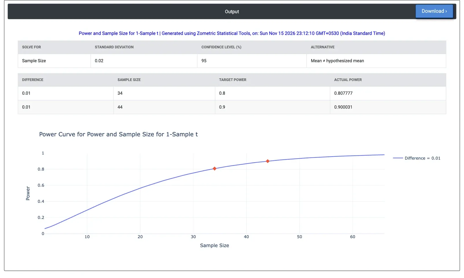
Figure 2 — Results for the example: 34 shafts for 80% power and 44 for 90% power to detect a 0.01 mm offset from nominal.
Worked Example
A turning cell makes shafts with a nominal diameter of 25.00 mm. After a tool change, the supervisor wants to check that the process is still centred, and an offset of 0.01 mm either way would matter. Past data put the standard deviation of the diameter at 0.02 mm. The supervisor leaves Sample sizes blank, enters Differences = 0.01, Power values = 0.8 0.9 and Standard deviation = 0.02, and keeps the two-sided alternative at 95% confidence.
The tool needs 34 shafts for 80% power (actual power 0.808) and 44 shafts for 90% power (actual power 0.900). The usual check of 20 shafts gives a power of only 0.565 for a 0.01 mm offset; with 20 shafts and 80% power the smallest offset the test can reliably detect is 0.0132 mm. If only an oversize shift matters (Mean > hypothesized mean), 27 shafts give 80% power.