
Power and Sample Size for 1-Sample Z
On this page
Purpose
Power and Sample Size for 1-Sample Z plans a test of one mean against a target when the process standard deviation is known, for example from a long, stable control chart history. It answers how many measurements are needed to detect a shift that matters, what power a planned sample gives, or the smallest shift a given sample can detect. Enter any two of sample size, difference and power, and the tool solves for the third. Use it before a 1-sample Z-test; if the standard deviation will be estimated from the sample, use Power and Sample Size for 1-Sample t instead.
Key Capabilities
- Solves for sample size, power or difference: leave blank the one you want.
- Several values at once, e.g. sample sizes “10 20 30”, give one row for each combination.
- Two-sided (Mean ≠ hypothesized mean) or one-sided (Mean < hypothesized mean, Mean > hypothesized mean) alternatives, at the confidence level you choose.
- Closed-form normal calculation, so results are exact for a known standard deviation.
- Power curve of power against sample size for each difference, with the solved points marked.
Statistical Methods
The test statistic is Z = (x̄ − μ₀) / (σ/√n) with σ treated as known, so the calculation uses the standard normal distribution throughout. The significance level is α = 1 − confidence level / 100, the standardised difference is d = difference / σ (the difference being the true mean minus μ₀), and z is z₁₋α/₂ for the two-sided alternative or z₁₋α for a one-sided one.
For a two-sided test, power = Φ(|d|·√n − z) + Φ(−|d|·√n − z); for Mean > hypothesized mean, power = Φ(d·√n − z), and for Mean < hypothesized mean, power = Φ(−d·√n − z), so a one-sided test has power near 0 for a difference on the wrong side. The sample size for a target power is n = ((z + z_β) / d)², where z_β is the normal quantile of the target power; n is rounded up and the power at that whole number is reported as the actual power. The smallest detectable difference for a given n and power is σ·(z + z_β)/√n, reported as a negative difference for the “less than” alternative.
Because σ is not estimated, the Z calculation gives slightly higher power than the t calculation at the same sample size, most noticeably for small samples. Use it only when the standard deviation really is known and stable. With a one-sided alternative, solving for sample size from a difference on the wrong side returns an error message.
Input Fields & Options
Field | Description |
Sample sizes | Space or comma-separated, e.g. “10 20 30”. Leave blank to solve for sample size. |
Differences | Space or comma-separated, e.g. “1 2 3”. The difference from the hypothesized mean you want to detect. Leave blank to solve for difference. |
Power values | Space or comma-separated, e.g. “0.8 0.9”. Leave blank to solve for power. |
Known standard deviation | Required. The population standard deviation, assumed known (not estimated from the sample). |
Confidence level | Default 95 (α = 0.05); 75 to 100. |
Alternative hypothesis | Mean ≠ hypothesized mean (default), Mean < hypothesized mean or Mean > hypothesized mean. |
Power curve | Ticked by default: draws power against sample size. |
Title | Title shown on the output and the power curve. |
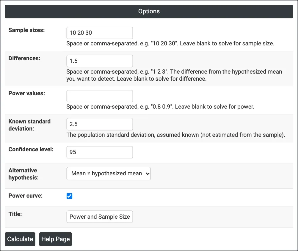
Figure 1 — Solving for power: Sample sizes = 10 20 30, Differences = 1.5, Known standard deviation = 2.5, two-sided at 95% confidence.
Output Descriptions
- Settings — what was solved for, the known standard deviation, the confidence level and the alternative hypothesis.
- Results — one row per combination: difference, sample size, and power when solving for power, target and actual power when solving for sample size, or difference when solving for difference.
- Power Curve — power against sample size for each difference, with the calculated points marked.
- PDF export via Download.
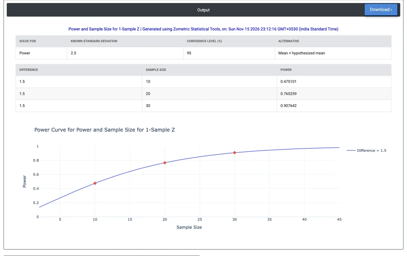
Figure 2 — Results for the example: power 0.475, 0.765 and 0.908 for 10, 20 and 30 packs at a 1.5 g shift.
Worked Example
A food packer audits the mean weight of 250 g packs. Years of stable control-chart data put the standard deviation at 2.5 g, so it is treated as known. A shift of 1.5 g in either direction would matter, and the audit team wants to compare samples of 10, 20 and 30 packs. They enter Sample sizes = 10 20 30, Differences = 1.5 and Known standard deviation = 2.5, leave Power values blank, and keep the two-sided alternative at 95% confidence.
The power is 0.475 with 10 packs, 0.765 with 20 and 0.908 with 30. A 10-pack audit would miss a real 1.5 g shift more than half the time, so the team moves to 30 packs; solving for sample size with Power values = 0.9 confirms that 30 packs are the minimum for 90% power. With 20 packs and 80% power the smallest shift detectable is 1.57 g. Had the standard deviation been estimated from each sample (the 1-Sample t calculation), the powers would be lower: 0.396, 0.721 and 0.888.