
Power and Sample Size for 2-Sample Equivalence Test
On this page
Purpose
Power and Sample Size for 2-Sample Equivalence Test plans a study that has to show two independent groups have practically the same mean, for example a second supplier against the current one, a new machine against an old one, or a cheaper material against the standard. You set an equivalence window for the difference (test mean − reference mean), and the tool tells you how many units each group needs to prove the difference lies inside it, what power a planned sample gives, or how large a true difference can be tolerated. Enter any two of sample size, difference and power, and the tool solves for the third. Use it before a 2-Sample Equivalence Test.
Key Capabilities
- Solves for sample size, power or difference: leave blank the one you want.
- Several values at once, e.g. differences “0 0.5” and power values “0.8 0.9”, give one row for each combination.
- Any equivalence window, symmetric or not.
- Exact power for the two one-sided tests (TOST) procedure with a pooled standard deviation and equal group sizes.
- Power curve of power against sample size for each difference, with the solved points marked.
Statistical Methods
The equivalence test uses two one-sided t-tests (TOST) on the difference of the two means. With n units in each group and a common standard deviation σ, the standard error of the difference is SE = σ·√(2/n) and the pooled t-tests have 2(n − 1) degrees of freedom. Equivalence is claimed when the difference is shown to be above the lower limit L and below the upper limit U, each one-sided test at significance level α (the Significance level (alpha) field, default 0.05).
Power is the probability that both one-sided tests succeed when the true difference is δ. It is computed exactly: for a given pooled sample standard deviation s the chance of success is Φ(−t·s/σ − (δ − U)/SE) − Φ(t·s/σ − (δ − L)/SE), with t = t₁₋α,2(n−1), and this is averaged over the chi-square distribution of the pooled variance by numerical integration. For sample size, the n per group that reaches the target power is found and rounded up, and the power at that n is reported as the actual power. When solving for the difference, the tool searches between the midpoint of the limits and the upper limit.
The difference to detect must lie strictly between the limits. Power is highest when the true difference is at the midpoint of the window and falls towards either limit. Compared with a one-sample study, two independent groups need about twice as many units per group, because both means carry sampling error.
Input Fields & Options
Field | Description |
Sample sizes | Per group. Space or comma-separated, e.g. “20 30 40”. Leave blank to solve for sample size. |
Difference(s) to detect | Space or comma-separated, e.g. “0.5 0.7”. The true difference (test mean − reference mean) you expect; must lie strictly between the limits. Leave blank to solve for it (searches between the midpoint of the limits and the upper limit). |
Power values | Space or comma-separated, e.g. “0.8 0.9”. Leave blank to solve for power. |
Lower equivalence limit / Upper equivalence limit | Required. The smallest and largest acceptable difference between the means; the lower limit must be less than the upper limit. |
Standard deviation | Required. Assumed or historical common (pooled) standard deviation of both populations. |
Significance level (alpha) | Default 0.05. Applied to each of the two one-sided tests. |
Power curve | Ticked by default: draws power against sample size. |
Title | Title shown on the output and the power curve. |
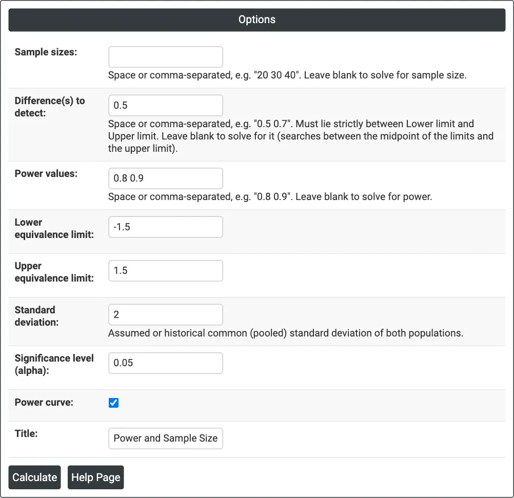
Figure 1 — Solving for sample size: Difference(s) to detect = 0.5, Power values = 0.8 0.9, limits −1.5 and 1.5, Standard deviation = 2, alpha = 0.05.
Output Descriptions
- Settings — what was solved for, the lower and upper equivalence limits, the standard deviation and the significance level.
- Results — one row per combination: difference, sample size per group, and target and actual power when solving for sample size, or power when solving for power, or difference when solving for difference.
- Power Curve — power against sample size for each difference, with the calculated points marked.
- PDF export via Download.
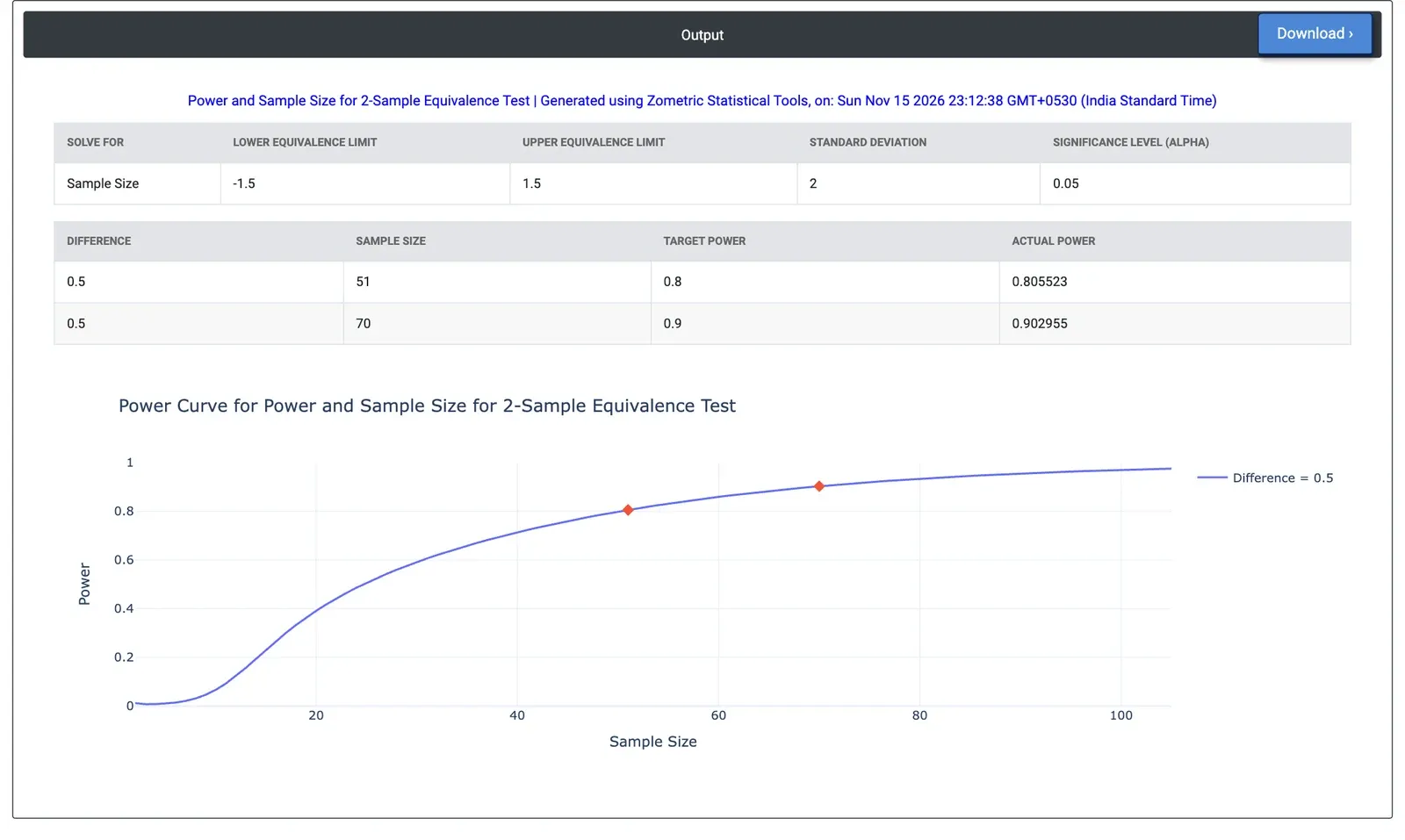
Figure 2 — Results for the example: 51 bars per supplier for 80% power and 70 for 90% power with a ±1.5 MPa window and a 0.5 MPa true difference.
Worked Example
A purchasing team wants to approve a second supplier of steel bar. The new supplier's mean yield strength must be within ±1.5 MPa of the current supplier's. Past data give a standard deviation of 2 MPa for both, and the team expects the true difference to be up to 0.5 MPa. They leave Sample sizes blank and enter Difference(s) to detect = 0.5, Power values = 0.8 0.9, Lower equivalence limit = −1.5, Upper equivalence limit = 1.5 and Standard deviation = 2, with alpha = 0.05.
The tool needs 51 bars from each supplier for 80% power (actual power 0.806) and 70 from each for 90% power (actual power 0.903). With 30 bars per supplier the power is only 0.591. If the suppliers really have the same mean (difference 0), 32 bars each give 80% power and 40 give 90%. Widening the window to ±2 MPa, if the design allows, cuts the requirement to 24 bars per supplier for 80% power at a 0.5 MPa difference.