
Power and Sample Size for 2-Sample Poisson Rate
On this page
Purpose
Power and Sample Size for 2-Sample Poisson Rate plans a comparison of two count rates, such as defects per roll on two lines, breakdowns per month before and after a maintenance change, or complaints per thousand deliveries from two depots. Enter any two of sample size, Rate 2 and power, and the tool solves for the third: how many units to observe in each group, what chance a planned sample gives of detecting the difference, or the Rate 2 that a given sample can detect. Use it before a 2-Sample Poisson Rate test.
Key Capabilities
- Solves for sample size, power or Rate 2: leave blank the one you want.
- Several values at once, e.g. Rate 2 values “2 3” and power values “0.8 0.9”, give one row for each combination.
- Separate observation lengths for the two samples, e.g. 1 hour per unit in Sample 1 and 2 hours in Sample 2.
- Two-sided (Rate 1 ≠ Rate 2) or one-sided (Rate 1 < Rate 2, Rate 1 > Rate 2) alternatives, at the confidence level you choose.
- Power curve of power against sample size for each Rate 2, with the solved points marked.
Statistical Methods
The tool uses a normal approximation for the difference of two Poisson rates, with the same number of units n in each group. Each unit in Sample 1 is observed for length t₁ and each unit in Sample 2 for length t₂, so the exposures are e₁ = n·t₁ and e₂ = n·t₂. The significance level is α = 1 − confidence level / 100, and z is z₁₋α/₂ for the two-sided alternative or z₁₋α for a one-sided one.
Under the null hypothesis the variance of the rate difference uses the exposure-weighted pooled rate λ̄ = (λ₁e₁ + λ₂e₂)/(e₁ + e₂): V₀ = λ̄·(1/e₁ + 1/e₂). Under the alternative it uses the two rates directly: V₁ = λ₁/e₁ + λ₂/e₂. Let Δ = λ₁ − λ₂ for Rate 1 > Rate 2, Δ = λ₂ − λ₁ for Rate 1 < Rate 2, and Δ = |λ₁ − λ₂| for the two-sided alternative. Power is Φ((Δ − z·√V₀) / √V₁). The sample size for a target power is found numerically and rounded up, and the power at that whole number is reported as the actual power. When solving for Rate 2, the tool searches above Rate 1 for Rate 1 < Rate 2 and for the two-sided alternative, and below it for Rate 1 > Rate 2.
Counts are assumed to follow a Poisson distribution with a constant rate per unit of observation. A one-sided test only has power when Rate 2 lies on the side the alternative names: with Rate 1 > Rate 2, a Rate 2 above Rate 1 gives a power near 0, and solving for sample size from it returns an error message. What drives power is the total exposure, so longer observation per unit needs fewer units.
Input Fields & Options
Field | Description |
Sample sizes | Per group. Space or comma-separated, e.g. “20 30 40”. Leave blank to solve for sample size. |
Rate 1 (baseline) | Required. The rate in the first group per unit of observation length, e.g. the current rate. |
Rate 2 value(s) | Space or comma-separated, e.g. “1.5 2”. The value(s) of Rate 2 you want to detect. Leave blank to solve for it. |
Power values | Space or comma-separated, e.g. “0.8 0.9”. Leave blank to solve for power. |
Observation length (Sample 1) | Default 1. Observation length (time, area, volume) per unit in Sample 1. |
Observation length (Sample 2) | Optional. Leave blank to use the same observation length as Sample 1. |
Confidence level | Default 95 (α = 0.05); 75 to 100. |
Alternative hypothesis | Rate 1 ≠ Rate 2 (default), Rate 1 < Rate 2 or Rate 1 > Rate 2. |
Power curve | Ticked by default: draws power against sample size. |
Title | Title shown on the output and the power curve. |
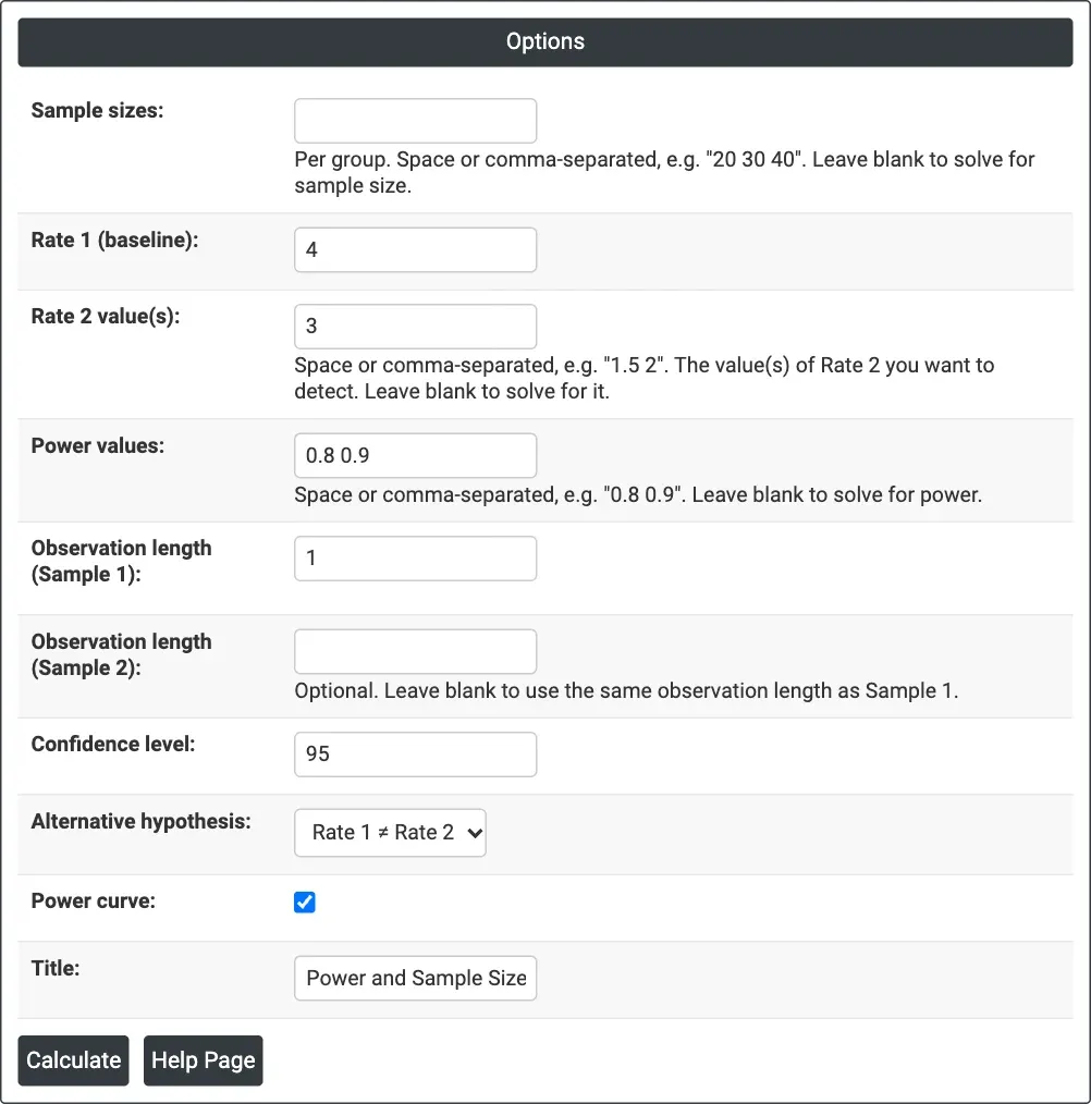
Figure 1 — Solving for sample size: Rate 1 (baseline) = 4, Rate 2 value(s) = 3, Power values = 0.8 0.9, observation length 1 for both samples, two-sided at 95% confidence.
Output Descriptions
- Settings — what was solved for, Rate 1 (baseline), the observation lengths of both samples, the confidence level and the alternative hypothesis.
- Results — one row per combination: Rate 2, sample size per group, and target and actual power when solving for sample size, or power when solving for power, or Rate 2 when solving for it.
- Power Curve — power against sample size for each Rate 2, with the calculated points marked.
- PDF export via Download.
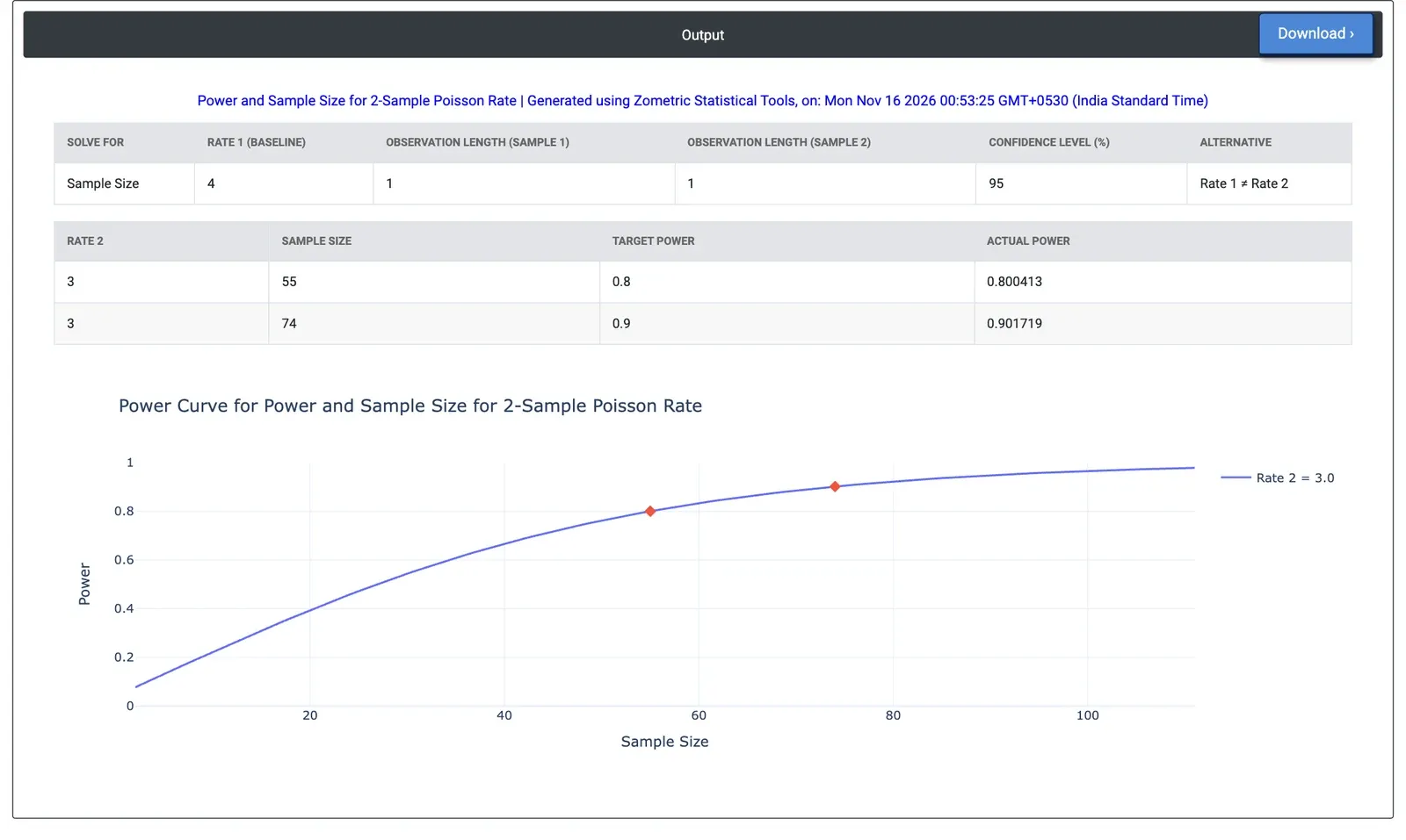
Figure 2 — Results for the example: 55 rolls per line for 80% power and 74 for 90% power to tell 4 defects per roll from 3.
Worked Example
A film extrusion plant averages 4 gel defects per roll on Line 1. Line 2 has a new filter and is expected to run at about 3 defects per roll. The quality engineer wants to know how many rolls to inspect from each line to confirm the difference. The engineer leaves Sample sizes blank and enters Rate 1 (baseline) = 4, Rate 2 value(s) = 3 and Power values = 0.8 0.9, with observation length 1 roll for both samples and the two-sided alternative at 95% confidence.
The tool needs 55 rolls per line for 80% power (actual power 0.800) and 74 per line for 90% power (actual power 0.902). Inspecting 30 rolls per line would give a power of 0.544. If each inspected unit is a double-length roll (Observation length = 2 for both samples), the requirement halves to 28 units per line for 80% power and 37 for 90%. A larger improvement, to 2 defects per roll, would be detected with 80% power from 12 rolls per line.