
Power and Sample Size for 2-Sample t
On this page
Purpose
Power and Sample Size for 2-Sample t plans a comparison of two means before you collect the data: how many units each group needs to detect a difference that matters, what chance (power) a planned sample size gives of detecting it, or the smallest difference a given sample size can detect. Enter any two of sample size, difference and power, and the tool solves for the third. Use it before a two-sample t-test, for example when comparing two suppliers, two machines or a process before and after a change.
Key Capabilities
- Solves for sample size, power or difference: leave blank the one you want.
- Several values at once, e.g. differences “3 5 7” and power values “0.8 0.9”, give one row for each combination.
- Two-sided (Mean 1 ≠ Mean 2) or one-sided (Mean 1 < Mean 2, Mean 1 > Mean 2) alternatives, at the confidence level you choose.
- When solving for sample size, reports the whole number of units per group and the actual power it gives.
- Power curve of power against sample size for each difference, with the solved points marked.
Statistical Methods
The calculation assumes two independent groups with the same sample size n per group and a common standard deviation σ, the same assumptions as the pooled two-sample t-test. The significance level is α = 1 − confidence level / 100, and the standardised difference is d = difference / σ.
Power is the probability that the t-test rejects the null hypothesis when the true difference is the one entered. It is computed from the noncentral t distribution with 2n − 2 degrees of freedom and noncentrality parameter δ = d·√(n / 2): for a two-sided test, power = P(T > t₁₋α/₂) + P(T < −t₁₋α/₂), where T follows that noncentral t. For sample size, the n that gives the target power is found and rounded up to the next whole number, and the power at that n is reported as the actual power. For difference, the smallest difference that reaches the target power with the given n is found.
Power rises with the sample size and the difference, and falls as the standard deviation grows or the confidence level rises. A one-sided test needs fewer units than a two-sided one for the same power, but only detects a difference in the stated direction.
Input Fields & Options
Field | Description |
Sample sizes | Per group. Space or comma-separated, e.g. “10 20 30”. Leave blank to solve for sample size. |
Differences | Space or comma-separated, e.g. “1 2 3”. The difference between the two means you want to detect, in the units of the measurement. Leave blank to solve for difference. |
Power values | Space or comma-separated, e.g. “0.8 0.9”. Leave blank to solve for power. |
Standard deviation | Required. Assumed or historical common (pooled) standard deviation of both populations, e.g. from past data or a pilot run. |
Confidence level | Default 95 (α = 0.05); 75 to 100. |
Alternative hypothesis | Mean 1 ≠ Mean 2 (default), Mean 1 < Mean 2 or Mean 1 > Mean 2. |
Power curve | Ticked by default: draws power against sample size. |
Title | Title shown on the output. |
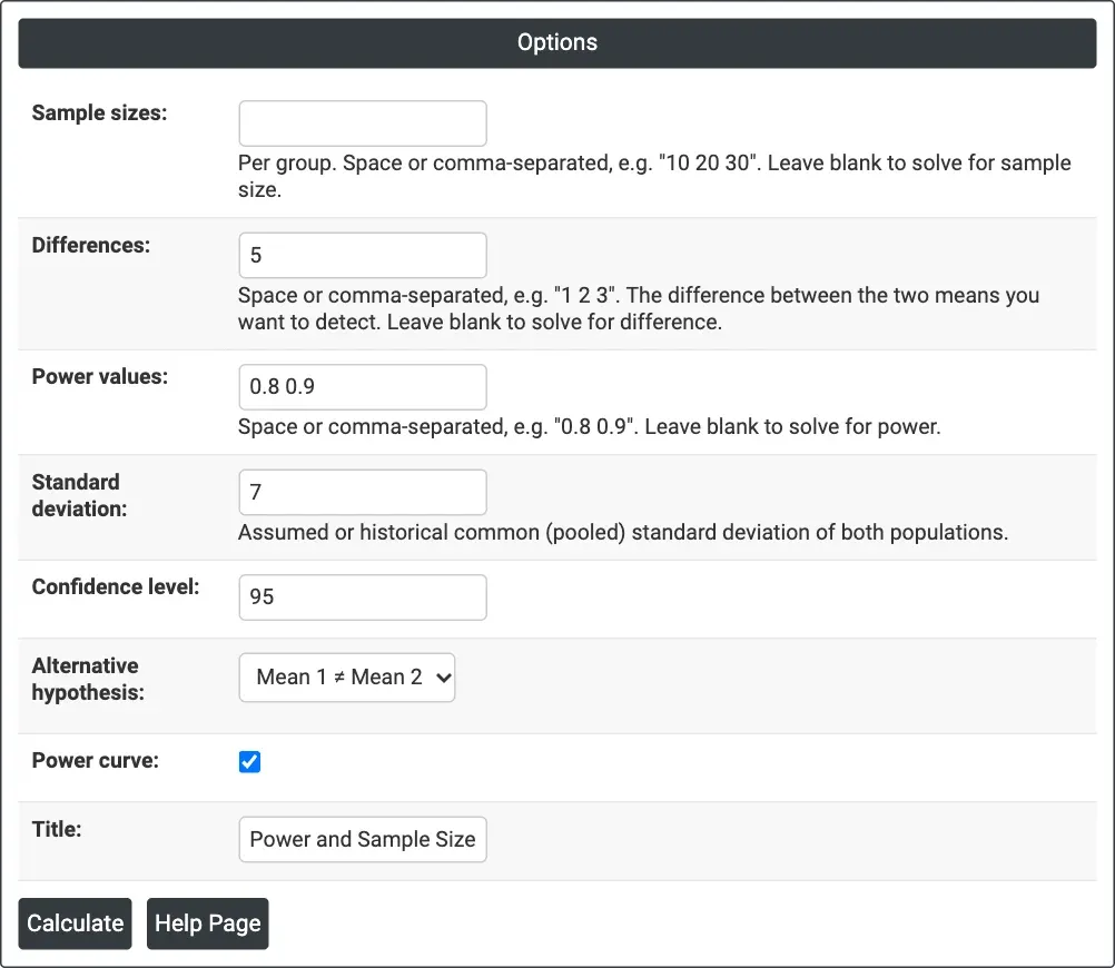
Figure 1 — Solving for sample size: Differences = 5, Power values = 0.8 0.9, Standard deviation = 7, two-sided at 95% confidence.
Output Descriptions
- Settings — what was solved for, the standard deviation, the confidence level and the alternative hypothesis.
- Results — one row per combination: difference, sample size (per group), and target and actual power when solving for sample size, or power when solving for power, or difference when solving for difference.
- Power Curve — power against sample size for each difference, with the calculated points marked.
- PDF export via Download.
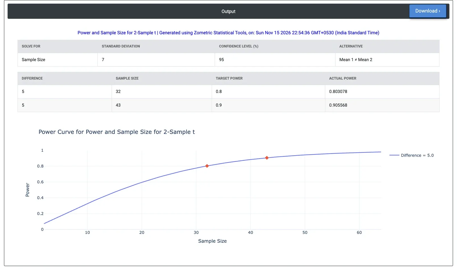
Figure 2 — Results for the example: 32 units per group for 80% power and 43 for 90% power, with the power curve for a difference of 5.
Worked Example
A quality team plans a trial to compare the mean tensile strength of parts from two suppliers. Past data put the standard deviation at 7 MPa, and a difference of 5 MPa between the suppliers would matter. They leave Sample sizes blank, enter Differences = 5, Power values = 0.8 0.9 and Standard deviation = 7, and keep the two-sided alternative at 95% confidence.
The tool needs 32 parts per group for 80% power (actual power 0.803) and 43 per group for 90% power (actual power 0.906). With only 20 parts per group the power would be 0.595: about a 40% chance of missing a real 5 MPa difference. Detecting a smaller difference of 4 MPa with 80% power needs 50 parts per group, and if only one direction matters (a one-sided alternative), 25 parts per group give 80% power for a 5 MPa difference.