
Power and Sample Size for One-Way ANOVA
On this page
Purpose
Power and Sample Size for One-Way ANOVA plans a comparison of the means of three or more groups, such as several furnaces, suppliers, operators or recipes. The size of the effect is entered as the maximum difference between any two group means that you want to detect. Enter any two of sample size per level, maximum difference and power, and the tool solves for the third: how many units each group needs, what power a planned design gives, or the largest-to-smallest gap a given design can detect. Use it before a One-Way ANOVA.
Key Capabilities
- Solves for sample size, power or maximum difference: leave blank the one you want.
- Several values at once, e.g. maximum differences “1.5 2” and power values “0.8 0.9”, give one row for each combination.
- Any number of levels from 2 upwards, with a balanced design (the same sample size in every level).
- When solving for sample size, reports the whole number per level and the actual power it gives.
- Power curve of power against sample size per level for each maximum difference, with the solved points marked.
Statistical Methods
The calculation assumes k independent groups from normal populations with a common standard deviation σ and n units per level (N = n·k in total). The significance level is α = 1 − confidence level / 100. To turn the maximum difference Δ into an effect size, the tool uses the arrangement of means that gives the least power for that Δ, as Minitab does: two levels at −Δ/2 and +Δ/2 and the other k − 2 levels at the grand mean. The effect size is f = σₘ/σ, where σₘ is the standard deviation of those k means, so σₘ² = Δ²/(2k).
Power is the probability that the ANOVA F-test rejects the hypothesis of equal means. It is computed from the noncentral F distribution with k − 1 and N − k degrees of freedom and noncentrality parameter λ = f²·N. For sample size, the total N that gives the target power is found, divided by k and rounded up per level, and the power at that size is reported as the actual power. For the maximum difference, the effect size that reaches the target power is found and converted back to Δ.
Because this is the least favourable arrangement, the answer is conservative: if the means are more spread out, for example two levels at each extreme, the real power is higher than reported and fewer units would do (see the worked example). With two levels there is only one arrangement.
Input Fields & Options
Field | Description |
Sample sizes | Per level (balanced design). Space or comma-separated, e.g. “10 20 30”. Leave blank to solve for sample size. |
Maximum difference between means | Space or comma-separated, e.g. “1 2 3”. The gap between the largest and smallest mean you want to detect. Leave blank to solve for the difference. |
Power values | Space or comma-separated, e.g. “0.8 0.9”. Leave blank to solve for power. |
Standard deviation | Required. Assumed or historical common standard deviation, same for every level. |
Number of levels | Required, at least 2. Number of groups being compared. |
Confidence level | Default 95 (α = 0.05); 75 to 100. |
Power curve | Ticked by default: draws power against sample size per level. |
Title | Title shown on the output and the power curve. |
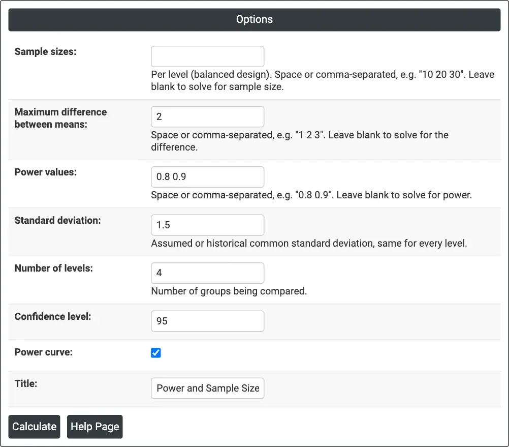
Figure 1 — Solving for sample size: Maximum difference between means = 2, Power values = 0.8 0.9, Standard deviation = 1.5, Number of levels = 4, at 95% confidence.
Output Descriptions
- Settings — what was solved for, the number of levels, the standard deviation and the confidence level.
- Results — one row per combination: maximum difference, sample size per level, and target and actual power when solving for sample size, or power when solving for power, or maximum difference when solving for it.
- Power Curve — power against sample size per level for each maximum difference, with the calculated points marked.
- PDF export via Download.
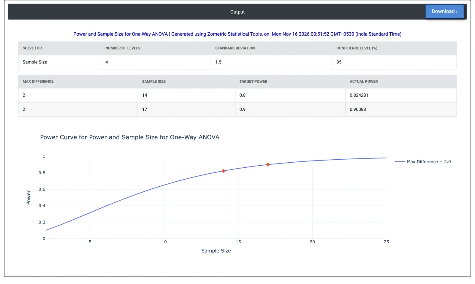
Figure 2 — Results for the example: 14 parts per furnace for 80% power (actual 0.824) and 17 for 90% power (actual 0.901).
Worked Example
A heat-treatment shop runs four furnaces and wants to check whether they give the same mean surface hardness. A gap of 2 HRC between the best and worst furnace would matter, and the hardness standard deviation within a furnace is about 1.5 HRC. The metallurgist leaves Sample sizes blank, enters Maximum difference between means = 2, Power values = 0.8 0.9, Standard deviation = 1.5 and Number of levels = 4, at 95% confidence.
The tool needs 14 parts per furnace for 80% power (actual power 0.824) and 17 per furnace for 90% power (actual power 0.901), so 56 and 68 parts in all. With 8 parts per furnace the power would be only 0.532, and with 5 parts 0.317. With 14 parts per furnace and 80% power, the smallest maximum difference the study can detect is 1.94 HRC. These figures assume the least favourable pattern: one furnace high, one low and the other two midway. If two furnaces sit at each extreme instead, 8 parts per furnace would already give a power of 0.852, so the plan errs on the safe side.