
Probability Plot
On this page
Purpose
The Probability Plot checks whether data follow a chosen distribution, most often the normal distribution. The ordered data are plotted on a scale on which the chosen distribution appears as a straight line: if the points follow the line, the distribution fits. Use it before capability analysis, control limits, tolerance intervals or t-tests that assume normality, and to choose a distribution (Weibull, lognormal, exponential) for reliability or non-normal capability work.
Key Capabilities
- Nine distributions: Normal, Lognormal, Weibull, Exponential, 2-Parameter Exponential, Smallest Extreme Value, Largest Extreme Value, Logistic and Loglogistic.
- Fitted reference line with pointwise confidence bounds at a chosen level (default 95%).
- Anderson-Darling (AD) statistic and its p-value in the legend for every distribution, so the fits can be compared.
- Several variables overlaid on one plot, or one variable split into groups by a By column, each with its own fitted line.
- Logarithmic data axis for the Lognormal, Weibull and Loglogistic, as on standard probability paper.
Statistical Methods
For each variable or group (at least 3 values), the data are sorted, x₍₁₎ ≤ … ≤ x₍ₙ₎, and each is given the plotting position pᵢ = (i − 0.3) / (n + 0.4), Benard's median-rank approximation. The vertical axis is the inverse CDF of the chosen distribution, labelled in percent, so a sample from that distribution falls close to a straight line. The reference line is the fitted CDF: for the Normal, the sample mean and the standard deviation (n − 1 divisor); for the other distributions, maximum likelihood, with the threshold fixed at 0 for the Lognormal, Weibull, Exponential and Loglogistic (these need positive values).
The confidence bounds are drawn through each point: at level C, the lower bound is the α/2 quantile of a Beta(i, n − i + 1) distribution and the upper bound the 1 − α/2 quantile of a Beta(i + 1, n − i) distribution, where α = 1 − C/100. Points that leave the bounds are evidence against the distribution.
The Anderson-Darling statistic AD = −n − (1/n) Σ (2i − 1)[ln F(x₍ᵢ₎) + ln(1 − F(x₍ₙ₊₁₋ᵢ₎))] measures how far the points are from the fitted CDF F, with extra weight in the tails; smaller is better. The legend shows this unadjusted AD for every distribution, as Minitab does. The p-value comes from a modified statistic, as in D'Agostino and Stephens: for the Normal and Lognormal (on the logs), AD·(1 + 0.75/n + 2.25/n²) converted with Stephens' approximation; for the Weibull and the two extreme value distributions, AD·(1 + 0.2/√n); for the Exponential, AD·(1 + 0.6/n); for the Logistic and Loglogistic, AD·(1 + 0.25/n). The last three are looked up in Stephens' tables of critical values and interpolated, so a p-value beyond the table is shown as a bound, such as >0.250 or <0.010. For the 2-Parameter Exponential the n − 1 gaps x₍ᵢ₎ − x₍₁₎ are tested as exponential. A p-value below 0.05 is evidence that the data do not follow the distribution; between distributions, the larger p-value usually means the closer fit.
Input Fields & Options
Field | Description |
Variables | Required. One numeric column, or several to overlay (a “Multiple” probability plot). |
By (grouping) column | Optional. One fitted line per group. Only used when a single variable is selected. |
Distribution | Normal (default), Lognormal, Weibull, Exponential, 2-Parameter Exponential, Smallest Extreme Value, Largest Extreme Value, Logistic or Loglogistic. |
Confidence level (%) | Default 95; 1 to 99.99. Level of the confidence bounds. |
Display confidence interval bounds | Ticked by default. Draws the bounds as dotted lines. |
Title | Title of the plot. Default “Probability Plot”. |
Data Options: Subset (optional) | Exclude matching rows (default) or Include only matching rows; Row numbers (e.g. 3,7,12-15) and/or a Condition (e.g. Tensile_Strength_MPa > 205) select the rows. |
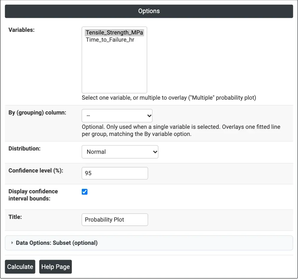
Figure 1 — Options for the example: Tensile_Strength_MPa on a Normal probability plot with 95% bounds.
Output Descriptions
- Probability Plot — the data (horizontal axis) against percent on the distribution's probability scale, with the fitted line and the dotted confidence bounds. The legend gives each series' AD statistic and its p-value.
- PDF export via Download.
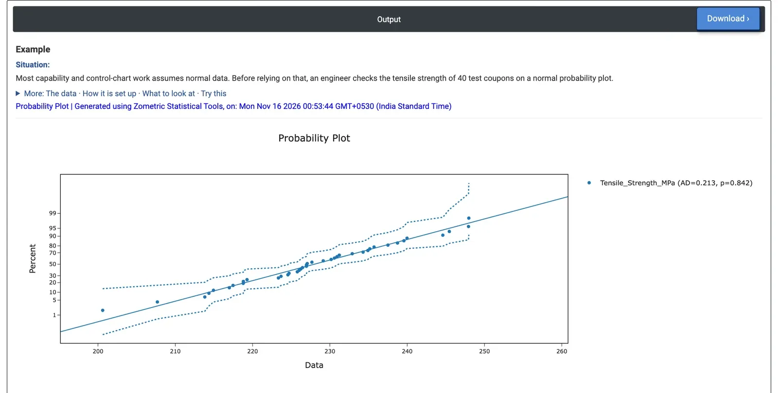
Figure 2 — Normal probability plot of the tensile strength of 40 coupons: AD = 0.213, p = 0.842.
Worked Example
Before setting control limits and calculating capability, an engineer checks whether the tensile strength of 40 test coupons can be treated as normal. Variables = Tensile_Strength_MPa, Distribution = Normal, Confidence level 95, bounds displayed.
The points follow the straight line and stay inside the dotted bounds over the whole range, from 200.61 to 247.97 MPa. The legend shows AD = 0.213 with p = 0.842, far above 0.05: there is no evidence against normality. The fitted line has mean 227.97 MPa and standard deviation 10.61 MPa, so normal-based capability and control-chart methods can be used. Points bending away from the line at either end would have pointed to a skewed or heavy-tailed distribution.
The same worksheet holds 40 times to failure (hours). Plotting Time_to_Failure_hr against several distributions gives AD = 0.210 with p > 0.250 for the Weibull (shape 3.23, scale 192.96 hours), AD = 0.158 with p = 0.947 for the Normal, AD = 1.228 with p < 0.005 for the Lognormal and AD = 7.628 with p < 0.010 for the Exponential. The Exponential, which assumes a constant failure rate, clearly does not fit, and neither does the Lognormal. The Weibull and Normal both fit well; for failure times the Weibull is the usual choice, since its shape above 1 describes wear-out and it cannot predict negative lives.