
Probit Analysis
On this page
Purpose
Probit Analysis models how the proportion of units that fail (or respond) rises with the level of a stress, from pass/fail tests run at several stress levels. Typical uses are drop tests, impact tests, burst-pressure or voltage step tests, and dose-response trials. It answers questions such as: at what drop height do half of the units crack, and at what height do 90% crack? The result gives a stress limit with a confidence interval, which can be compared with a specification or a field condition.
Key Capabilities
- Works with grouped pass/fail data: the number of units tested and the number that failed at each stress level.
- Normal (probit) or Logistic (logit) tolerance distribution.
- Fit against ln(stress), the usual choice for physical stresses, or against stress itself.
- Coefficient table with Z tests for the intercept and slope.
- Stress at which any chosen percentages of units fail, with confidence intervals, and a probit plot of observed against fitted.
Statistical Methods
At each stress level s, r of n units respond. The model assumes that each unit has its own tolerance, the stress at which it fails, and that these tolerances follow a Normal or Logistic distribution in x, where x = ln(s) when Fit against ln(stress) is ticked and x = s otherwise. The probability of failing at stress s is then P = G(b₀ + b₁·x), where G is the standard normal (probit link) or standard logistic (logit link) cumulative distribution function. The counts are fitted as a binomial generalised linear model by maximum likelihood, and the intercept b₀ and slope b₁ are tested with Wald Z statistics. A slope significantly greater than 0 means the failure proportion rises with stress.
The stress at which p% of units fail is found from G⁻¹(p/100) = b₀ + b₁·x, so x_p = (G⁻¹(p/100) − b₀) / b₁, and s_p = exp(x_p) on the log scale. Its confidence interval is computed with the delta method: the variance of x_p comes from the covariance matrix of b₀ and b₁, the interval x_p ± z·SE is formed, and on the log scale both ends are converted back with exp, so the interval is not symmetric. Normal and Logistic usually give similar answers near 50% and differ more in the tails.
The probit plot shows each stress level's observed proportion on a probability scale against stress (log scale when fitting against ln(stress)), with the fitted straight line. Points close to the line mean the model fits. A level where no unit or every unit failed has no finite position on the probability scale, so, as in Minitab, it is left off the plot (it is still used in the fit) and a note below the plot says how many rows were left off.
Input Fields & Options
Field | Description |
Response (number of events) | Required. Number of units that failed or responded at each stress level. Cannot exceed Trials. |
Trials (number of tests) | Required. Number of units tested at each stress level. |
Stress (predictor) | Required. The stress level of each row. At least 3 rows are needed. |
Fit against ln(stress) | Ticked by default. Standard for physical stress and dose variables; stress must then be positive. Untick if stress should stay on a linear scale. |
Distribution | Normal (probit link) (default) or Logistic (logit link). |
Percent levels | Comma-separated percents to report the effective stress for. Default 50, 90, 95. |
Confidence level (%) | For the intervals on the effective stress. Default 95; 50 to 99.99. |
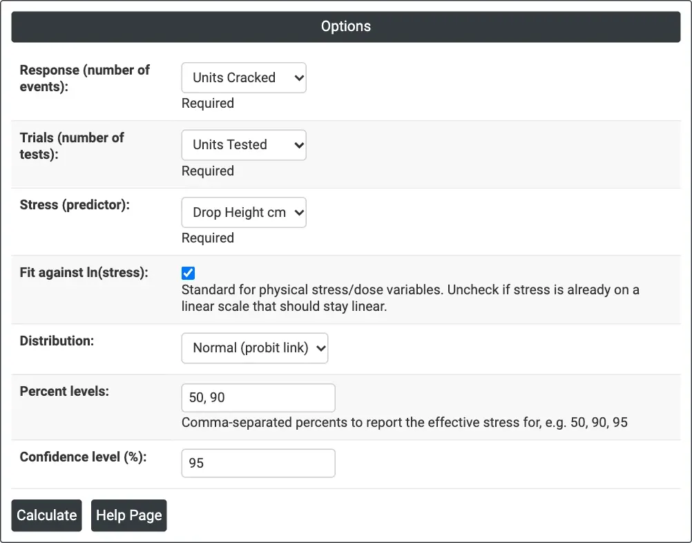
Figure 1 — Options for the drop-test example: cracked and tested counts at each drop height, fitted against ln(height) with the Normal distribution, percent levels 50 and 90.
Output Descriptions
- Coefficients — Intercept and Slope with Coef, SE Coef, Z and P.
- Percent table — for each percent level, the Stress at which that percent of units fail, with lower and upper confidence limits.
- Probit Plot — observed proportion at each stress level on a probability scale (Percent), with the fitted line.
- PDF export via Download.
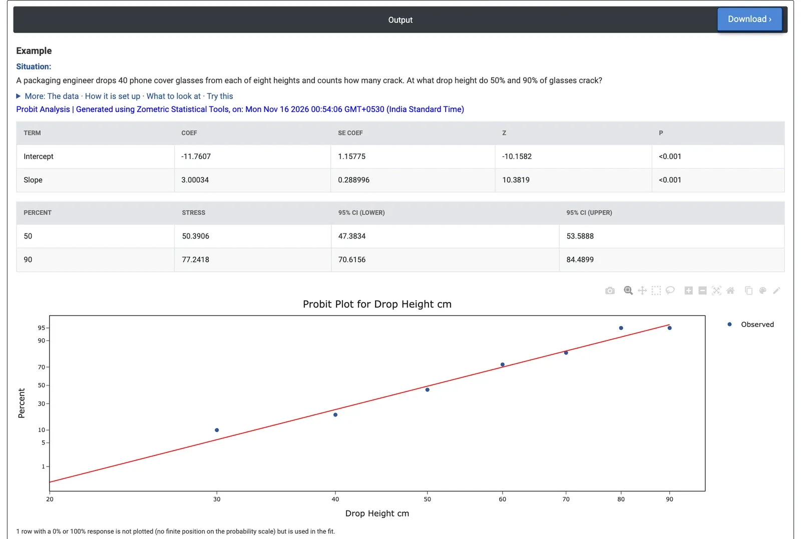
Figure 2 — Drop-test results: 50% of glasses crack at 50.4 cm (95% CI 47.4 to 53.6) and 90% at 77.2 cm (70.6 to 84.5).
Worked Example
A packaging engineer drops 40 phone cover glasses from each of eight heights, from 20 to 90 cm, and counts how many crack. The share cracked rises from none at 20 cm (the one level left off the probit plot) to 45% (18 of 40) at 50 cm and 95% (38 of 40) at 80 and 90 cm. The engineer wants to know the heights at which 50% and 90% of glasses crack. They set Response = Units Cracked, Trials = Units Tested, Stress = Drop Height cm, keep Fit against ln(stress) ticked and Distribution = Normal, and enter Percent levels = 50, 90.
The slope on ln(height) is 3.000 (Z = 10.38, p < 0.001), so drop height clearly drives cracking. Half of the glasses are expected to crack at 50.4 cm (95% CI 47.4 to 53.6 cm), and 90% at 77.2 cm (95% CI 70.6 to 84.5 cm). The interval at 90% is wider because it lies further from the middle of the data. Adding 10 to the percent levels gives 32.9 cm (29.4 to 36.8 cm): below about 30 cm few glasses crack.
With the Logistic distribution the answers are almost the same: 50.7 cm for 50% and 76.9 cm for 90%. Fitting against height rather than ln(height) moves the 50% point to 53.2 cm, so the choice of scale matters more than the choice of distribution here. For the packaging team, these heights are the figures to compare with the drop heights the packed glass must survive in handling: if no more than about 10% cracking is acceptable, the glass alone should not see the equivalent of a drop above about 33 cm.