
Random Data
On this page
Purpose
Random Data generates random numbers from one of 26 distributions and puts them in the data pane, ready to copy or to use in other tools. Use it to make practice data for training, to see how much a sample from a known process varies (a histogram of 30 values from a perfect normal process is rarely bell-shaped), to try out an analysis before the real data arrive, or to simulate a process for a what-if study, for example cycle times from a triangular estimate or failure times from a Weibull model. An optional graphical summary describes the numbers you generated.
Key Capabilities
- 26 distributions in one Distribution list: continuous (Normal, Lognormal, Weibull, Exponential, Gamma, Uniform, Triangular and others), discrete (Binomial, Poisson, Geometric, Hypergeometric, Integer, Discrete and others) and Multivariate Normal.
- Only the parameter fields of the chosen distribution are shown.
- 10 to 10,000 rows and 1 to 10 independent columns (data_1, data_2, …).
- Optional rounding to a set number of decimals.
- Optional graphical summary of all generated values: histogram, summary statistics, Anderson-Darling normality test, confidence intervals and probability plot.
- Multivariate Normal: correlated columns from a vector of means and a covariance matrix, with the sample correlation and covariance matrices as a check.
Statistical Methods
Values are drawn independently with NumPy and SciPy random number generators, with no fixed seed, so every Calculate gives new numbers. Each column is a separate sample of the chosen size from the same distribution. Parameters follow the usual definitions: for example Normal (mean μ, standard deviation σ), Weibull (shape β, scale η, optional threshold added to every value), Exponential (scale = mean, optional threshold), Integer (whole numbers from Minimum to Maximum, both included), Geometric (number of trials up to and including the first event) and Negative Binomial (number of non-events before the required number of events). For Lognormal you enter the mean and standard deviation of the data themselves: the tool converts them to the log-scale parameters σ = √ln(1 + (s/m)²) and μ = ln(m) − σ²/2. For Discrete, the probabilities are rescaled to sum to 1.
With Graphical Summary ticked, all columns are pooled into one sample and described: mean, standard deviation, variance, skewness, kurtosis, N, minimum, quartiles, median, maximum and coefficient of variation (%); the Anderson-Darling test of normality (A-squared and p-value); 95% confidence intervals for the mean (t), the median (Hettmansperger-Sheather) and the standard deviation (chi-square). With Exclude outliers ticked, values outside Q1 − 1.5×IQR or Q3 + 1.5×IQR are left out of the summary only; the generated data keep them. For Multivariate Normal, the covariance matrix must be square, symmetric, positive semi-definite and match the number of means.
Input Fields & Options
Field | Description |
Distribution | Required. One of 26 distributions; the parameter fields below change with it. |
Number of rows of data to generate | Required, 10 to 10,000. |
Number of columns | Default 1, up to 10. Each column is an independent sample. Not used for Multivariate Normal (one column per mean). |
Graphical Summary | Unticked by default. Adds the graphical summary of the generated values to the output. |
Exclude outliers (1.5×IQR rule) | Optional. Has no effect unless Graphical Summary is checked; then it removes outliers from the summary only. |
Decimals | Optional, 0 to 10. Rounds the generated values for the continuous distributions (Normal, Lognormal, Weibull, Exponential, T, F, Beta, Cauchy, Chi-Square, Gamma, Laplace, the extreme value distributions, Logistic, Loglogistic, Triangular and Uniform). For Normal, at least enough decimals to show the standard deviation are kept. Not shown for the distributions that give whole numbers or listed values (Binomial, Poisson, Bernoulli, Discrete, Geometric, Hypergeometric, Integer and Negative Binomial) or for Multivariate Normal. |
Mean / Standard Deviation | Normal; Lognormal (mean and standard deviation of the data); Poisson uses Mean only. |
Number of trials / Event probability | Binomial. Event probability alone: Bernoulli and Geometric; with Number of events (required successes): Negative Binomial. |
Shape parameter / Scale parameter / Threshold parameter | Weibull (threshold optional); Gamma and Loglogistic use shape and scale. |
Scale parameter / Threshold parameter | Exponential (threshold optional). |
Location parameter / Scale parameter | Cauchy, Laplace, Largest Extreme Value, Smallest Extreme Value and Logistic. |
Degrees of freedom / Numerator and Denominator degrees of freedom | T and Chi-Square; F. |
First shape parameter / Second shape parameter | Beta. |
Values / Probabilities | Discrete. Comma or space-separated, same count, e.g. “1 2 3” and “0.2 0.3 0.5” (renormalized if they don't sum to 1). |
Population size (N) / Event count in population / Sample size (n) | Hypergeometric. The event count and the sample size cannot exceed the population size. |
Minimum / Maximum / Mode (most likely value) | Integer (minimum and maximum); Triangular (all three, mode between them). |
Lower endpoint / Upper endpoint | Uniform. |
Means / Covariance matrix | Multivariate Normal. Means one per variable, e.g. “10 20 30”; covariance rows separated by semicolons, e.g. “4,2,0; 2,9,1; 0,1,1”. |
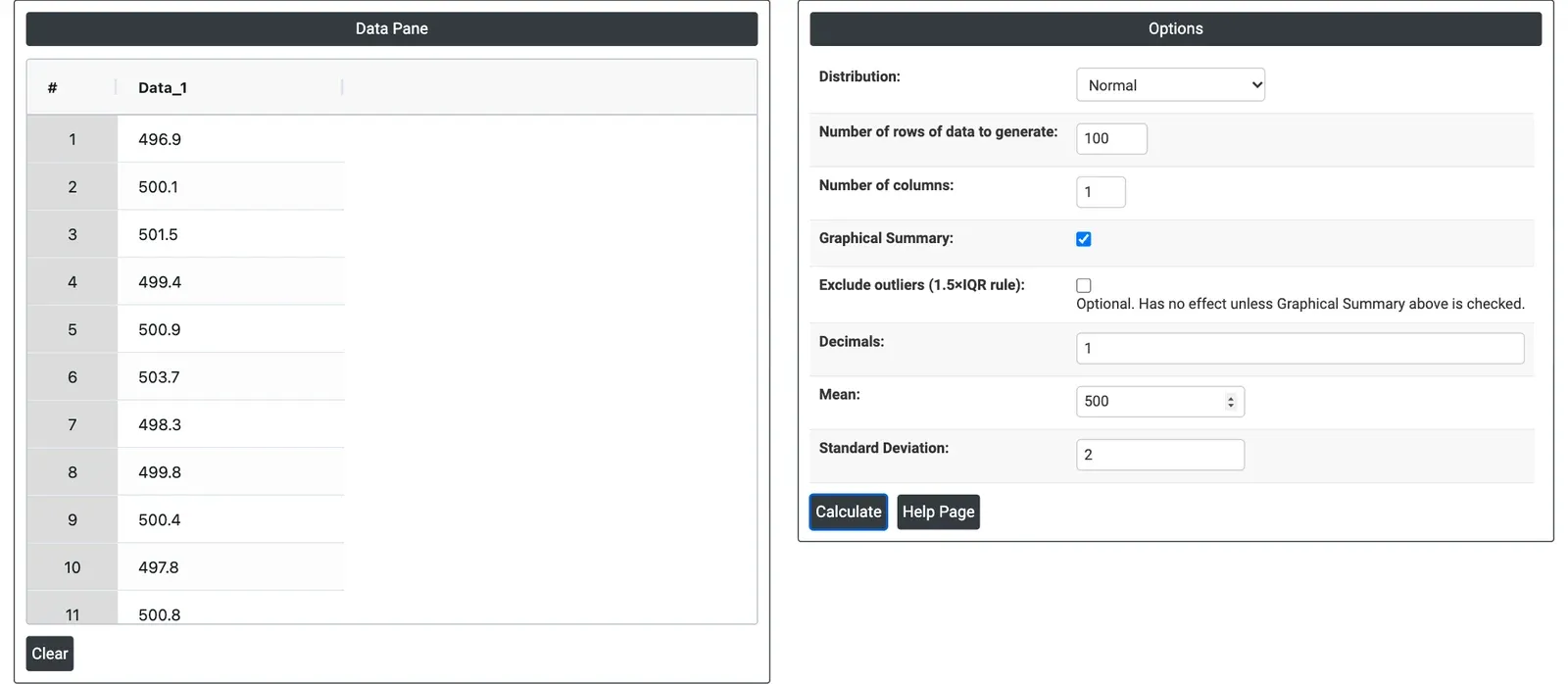
Figure 1 — 100 values from a Normal distribution with mean 500 and standard deviation 2, rounded to 1 decimal, in the data pane (left) with the Options (right).
Output Descriptions
- Data Pane — the generated values, one column per sample (data_1, data_2, …), replacing what was there.
- Graphical summary (when ticked) — histogram with fitted normal curve and box plot; summary table with A-Squared, p-value, Mean, StDev, Variance, Skewness, Kurtosis, N, Minimum, 1st Quartile, Median, 3rd Quartile, Maximum and Coeff Var; 95% Confidence Intervals plot for the mean and median; Probability Plot with the Anderson-Darling result; and a table of lower and upper 95% limits for the mean, median and standard deviation, with the half-width of each interval.
- Multivariate Normal — sample correlation and covariance matrices of the generated columns.
- PDF export via Download as PDF.
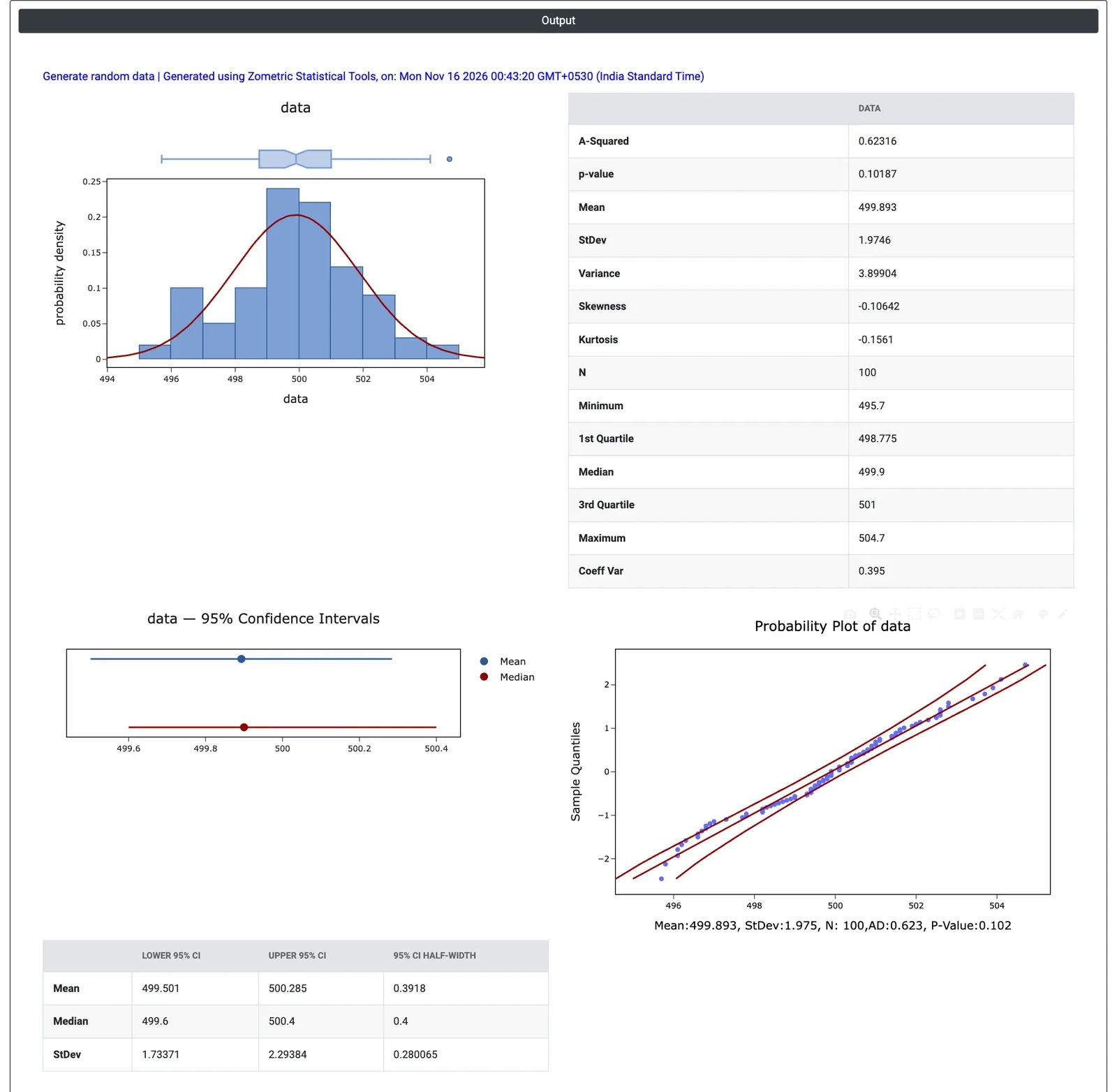
Figure 2 — Graphical summary of the 100 generated values: mean 499.89, StDev 1.97, Anderson-Darling p-value 0.102.
Worked Example
A quality trainer prepares a session on process variation for filling-line operators. The line fills 500 g bottles with a standard deviation of about 2 g. To show what normal variation alone looks like, the trainer chooses Distribution = Normal, Number of rows = 100, Number of columns = 1, Mean = 500, Standard Deviation = 2 and Decimals = 1, and ticks Graphical Summary.
The 100 simulated fill weights run from 495.7 to 504.7 g, with mean 499.89 g and standard deviation 1.97 g, not exactly 500 and 2 even though the process was set exactly. The histogram is lumpy rather than a clean bell curve, yet the Anderson-Darling test gives p = 0.102, so there is no evidence against normality. The 95% confidence interval for the mean, 499.50 to 500.29 g (half-width 0.39 g), contains the true 500, and the interval for the standard deviation, 1.73 to 2.29 g, contains the true 2.
The point for the operators: a stable, centred process still produces single bottles 4 g from target and sample statistics that differ from the true values. Each Calculate draws a new sample with slightly different numbers, which the trainer can use to show sample-to-sample variation. Generating 5 columns of 20 rows gives five small samples to compare, or the data can be copied into a capability or control chart tool for practice.