
Regression with Life Data
On this page
Purpose
Regression with Life Data relates product life to one or more numeric factors, such as load, temperature, voltage or a design dimension, when some units have not failed by the end of the test (right-censored). It fits a Weibull life model in which the characteristic life changes with the factors, so you can see how strongly each factor shortens or extends life and predict life at other settings. Use it for life tests run at several combinations of conditions, rather than at the levels of a single stress.
Key Capabilities
- Weibull accelerated failure time model with one or more numeric covariates.
- Handles right-censored units: tests stopped before failure.
- Coefficients with standard errors, Z tests, p-values and confidence intervals.
- Common Weibull shape with its estimate and interval.
- Log-likelihood and AIC for comparing models, and a survival plot at the average covariate values.
Statistical Methods
The model assumes that life follows a Weibull distribution with a common shape β and a scale (characteristic life, the time by which 63.2% fail) that depends on the covariates: ln(η) = b₀ + b₁Z₁ + b₂Z₂ + .... This is an accelerated failure time model: a change in a covariate stretches or shrinks the whole life distribution by a factor. A one-unit increase in Zⱼ multiplies life by exp(bⱼ), so a negative coefficient means shorter life. For a change of k units, the factor is exp(k · bⱼ).
The shape and coefficients are estimated together by maximum likelihood. A failure contributes the Weibull density at its time and a censored unit the Weibull survival probability exp(−(t/η)^β). Standard errors come from the inverse of the Hessian of the negative log-likelihood at the estimate (the observed information), computed numerically. Each coefficient is tested with Z = coef / SE against the standard normal distribution, and confidence intervals are coef ± z·SE at the chosen confidence level. AIC = 2k − 2 × log-likelihood, where k is the number of parameters; a lower AIC means a better model once the number of terms is allowed for, so compare AIC to decide whether a covariate is worth keeping.
The shape β describes how the failure rate changes with age: above 1 it rises (wear-out, as in fatigue), near 1 it is constant, and below 1 it falls. In the censoring column, rows equal to the censoring value are right-censored and every other row is a failure. The survival plot shows exp(−(t/η)^β) for a unit with each covariate at its sample mean.
Input Fields & Options
Field | Description |
Time variable | Required. Time or cycles to failure, or to censoring for units that did not fail. |
Use censoring column | Required. Rows equal to the censoring value are right-censored; every other row is a failure. Every row needs a value. |
Censoring value | The value in the censoring column that marks a unit still running when the test stopped. Default 0, so 1 = failure. |
Covariates (predictors) | One or more numeric predictor columns. Hold Ctrl or Command to select several. |
Confidence level (%) | For the intervals on the coefficients and the shape. Default 95; 50 to 99.99. |
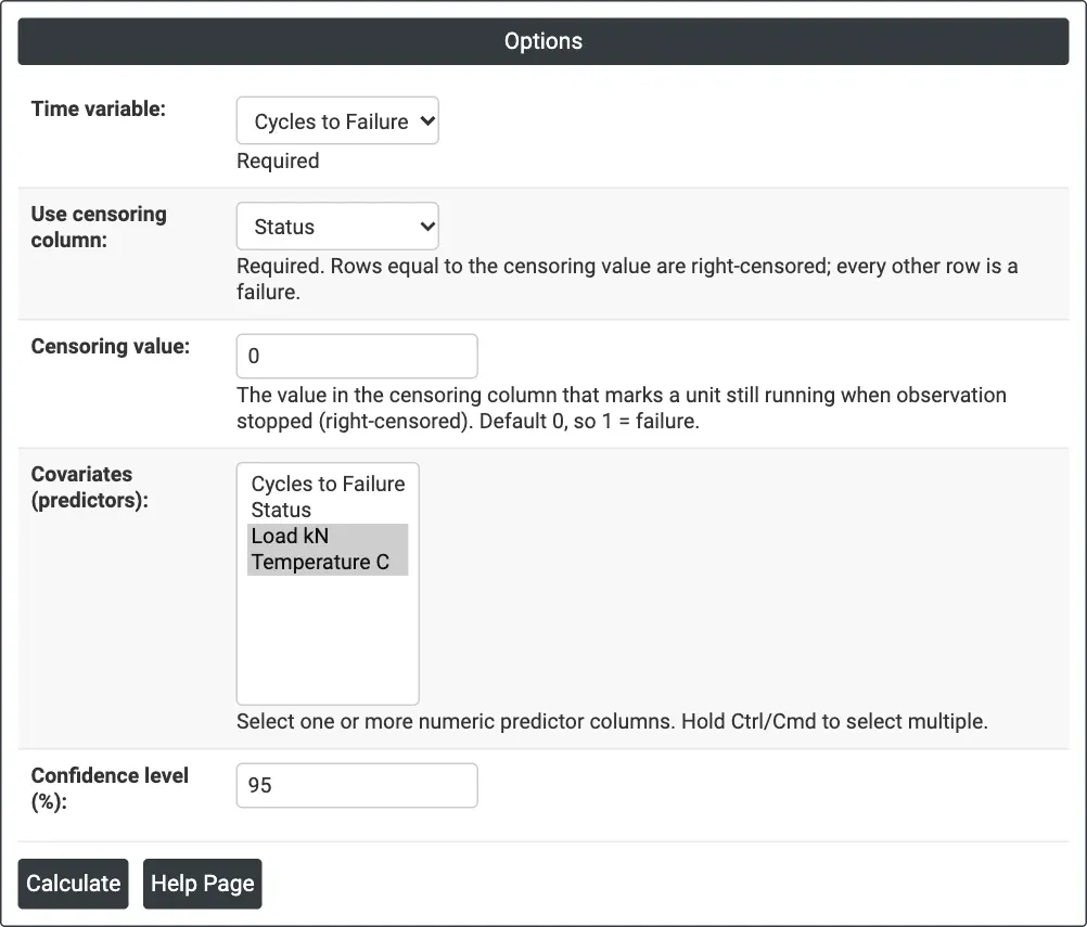
Figure 1 — Options for the spring example: cycles to failure, Status as the censoring column (0 = survived), load and temperature as covariates.
Output Descriptions
- Model summary — Distribution (Weibull (AFT)), Log-Likelihood, AIC, N (Observations) and N (Events), the number of failures.
- Shape table — Shape (Weibull) with its estimate, standard error and confidence limits.
- Coefficients — Intercept and each covariate with Coef, SE Coef, Z, P and confidence limits.
- Regression with Life Data Survival Plot (at mean covariate values) — fitted survival probability against time for a unit at the average of each covariate.
- PDF export via Download.
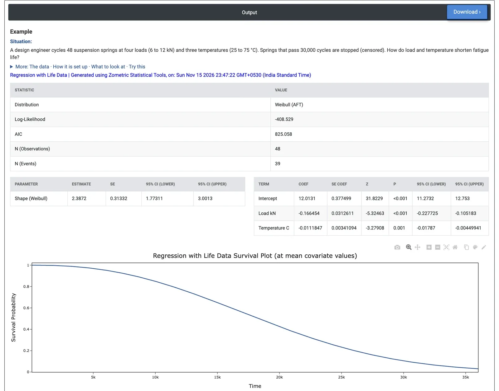
Figure 2 — Spring fatigue results: load coefficient −0.166 per kN and temperature coefficient −0.0112 per °C, Weibull shape 2.39 (95% CI 1.77 to 3.00), with the survival curve at the average load and temperature.
Worked Example
A design engineer cycles 48 suspension springs at four loads (6, 8, 10 and 12 kN) and three temperatures (25, 50 and 75 °C). Springs that pass 30,000 cycles are stopped and are right-censored; 39 of the 48 fail. The engineer wants to know how much load and temperature shorten fatigue life. They set Time variable = Cycles to Failure, Use censoring column = Status with Censoring value = 0, and select Load kN and Temperature C as covariates.
The load coefficient is −0.166 per kN (SE 0.0313, Z = −5.32, p < 0.001): each extra kN multiplies life by exp(−0.166) = 0.85, about 15% shorter, and the 95% confidence interval (−0.228 to −0.105) puts that factor between 0.80 and 0.90. The temperature coefficient is −0.0112 per °C (SE 0.00341, Z = −3.28, p = 0.001; 95% CI −0.0179 to −0.0045): each 10 °C hotter multiplies life by 0.89, and going from 25 to 75 °C cuts life to 57%. Both effects are significant. The common Weibull shape is 2.39 (95% CI 1.77 to 3.00), well above 1, so the failure rate rises with cycles: wear-out, as expected for fatigue.
From the fitted model, the characteristic life is about 45,900 cycles at 6 kN and 25 °C but only about 9,670 cycles at 12 kN and 75 °C. The survival plot shows a spring at the average test conditions (8.75 kN and 52.6 °C). Removing Temperature C from the covariates raises the AIC from 825.1 to 833.3, so the model with temperature is better. For the design, load has the larger effect over the tested ranges, but a spring that runs hot needs extra margin on load.