
Single Exponential Smoothing
On this page
Purpose
Single Exponential Smoothing smooths a time series with one running level that is updated each period by a share of the latest error, and forecasts that level for every future period. It suits a series that wanders around a fairly steady value with no clear trend or season, such as weekly demand for a mature spare part, a daily scrap rate or the fill weight of a stable line. For data with a trend use Double Exponential Smoothing; for data with a season use Winters' Method or Decomposition.
Key Capabilities
- Smoothing weight (alpha) that you specify, or the optimal weight from an ARIMA(0,1,1) fit when left blank.
- Starting value from the data or one you enter.
- Forecasts with prediction limits at the confidence level you choose, from the end of the series or from an earlier row to test the method against known data.
- MAPE, MAD and MSD accuracy measures, and a plot of the data, fits and forecasts.
- Optional results table (smoothed value, prediction and error for every period) and four-in-one residual plots.
Statistical Methods
The smoothed value is Sₜ = α·yₜ + (1 − α)·Sₜ₋₁. The fit (one-step-ahead prediction) for period t is Sₜ₋₁, the smoothed value at the end of the period before, and the error is yₜ minus that fit. A small α (e.g. 0.1–0.3) gives a smooth line that reacts slowly; a large α follows the latest values closely.
With a specified weight, the starting value S₀ is the mean of the first K observations (K = 6 by default). When the weight is left blank, the tool fits an ARIMA(0,1,1) model to the first differences by least squares and sets α = 1 − θ, where θ is the MA coefficient; the starting value then comes from that fit. This optimal α can come out above 1, which means the level overreacts to each new value; treat that as a sign the series has a trend. With Starting values = User-specified, the Initial level you enter is used as S₀.
All forecasts equal the last smoothed value at the forecast origin. The prediction limits are forecast ± z × 1.25 × MAD, where z is the normal quantile for the confidence level and MAD is the mean absolute error of the fits; they have the same width for every period ahead. Accuracy: MAPE = mean |error / data| × 100, MAD = mean |error|, MSD = mean error². The series must have no gaps and at least 4 values.
Input Fields & Options
Field | Description |
Variable (Y) | Required. The numeric series, in time order. |
Weight to use in smoothing (alpha) | 0.0001 to 1. Leave empty to use the optimal ARIMA(0,1,1) weight. |
Starting values | From the data (default): the optimal weight starts from the ARIMA fit; a specified weight from the mean of the first K observations. Or User-specified. |
Initial level | Used when Starting values is User-specified (required then). |
Initial smoothed value: average of first K observations, K = | Default 6. Active when a weight is entered. |
Number of forecasts | Default 0 (none), up to 1000. |
Confidence level (%) for forecast interval | Default 95. Active when forecasts are requested. |
Forecast origin (row) | Optional, active when forecasts are requested. Forecasts start after this row, using the data up to it; blank = end of the series. |
Results to display | Summary table (default) or Summary table and results table. |
Residual plots (four in one) | Unticked by default. Normal probability plot, residuals versus fits, histogram and residuals versus order. |
Title | Title of the output. Default Single Exponential Smoothing. |
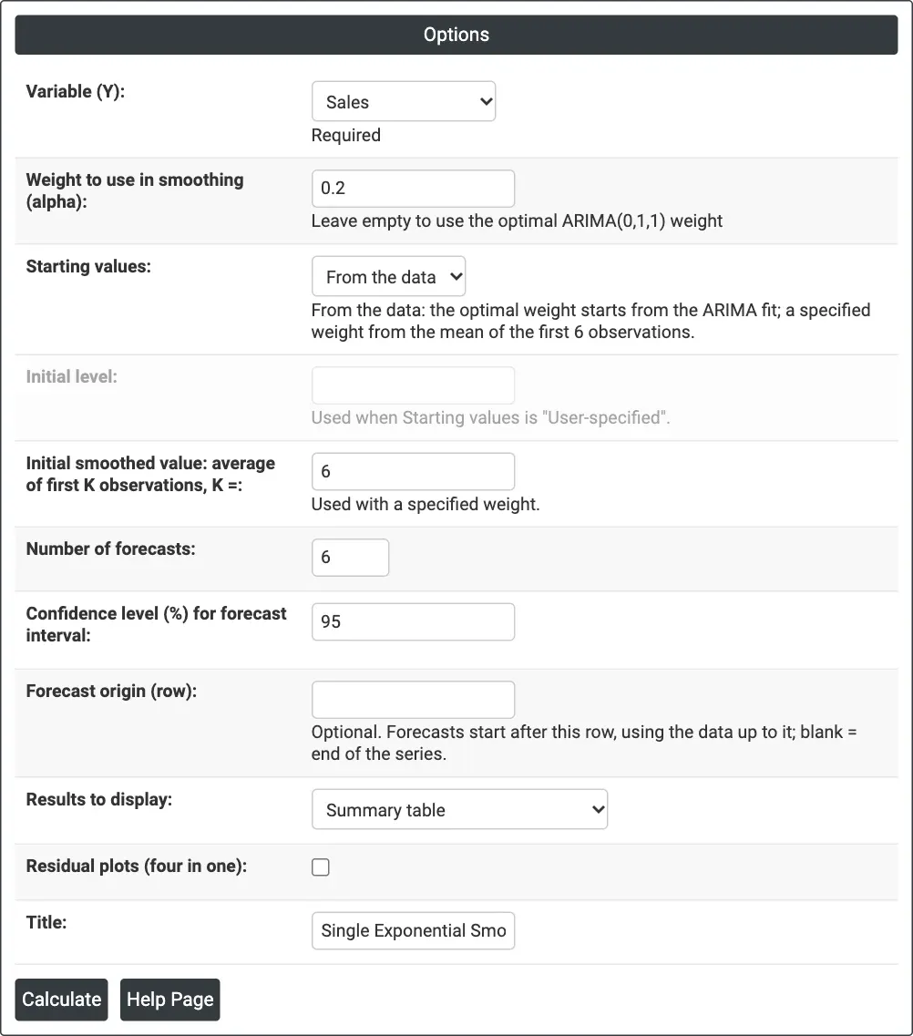
Figure 1 — Monthly Sales smoothed with alpha = 0.2 and six forecasts.
Output Descriptions
- Single Exponential Smoothing (graph) — actual data, fits, forecasts and the prediction band, with MAPE, MAD and MSD in the title and the weight used above the plot.
- Method — data column, length and whether the weight was specified or optimal (plus the forecast origin when set).
- Smoothing Constants — the value of α used.
- Accuracy Measures — MAPE, MAD and MSD.
- Forecasts — period, forecast, lower and upper limits.
- Results — when chosen: Period, data, Smooth, Predict and Error for each period.
- Residual Plots — when ticked.
- PDF export via Download.
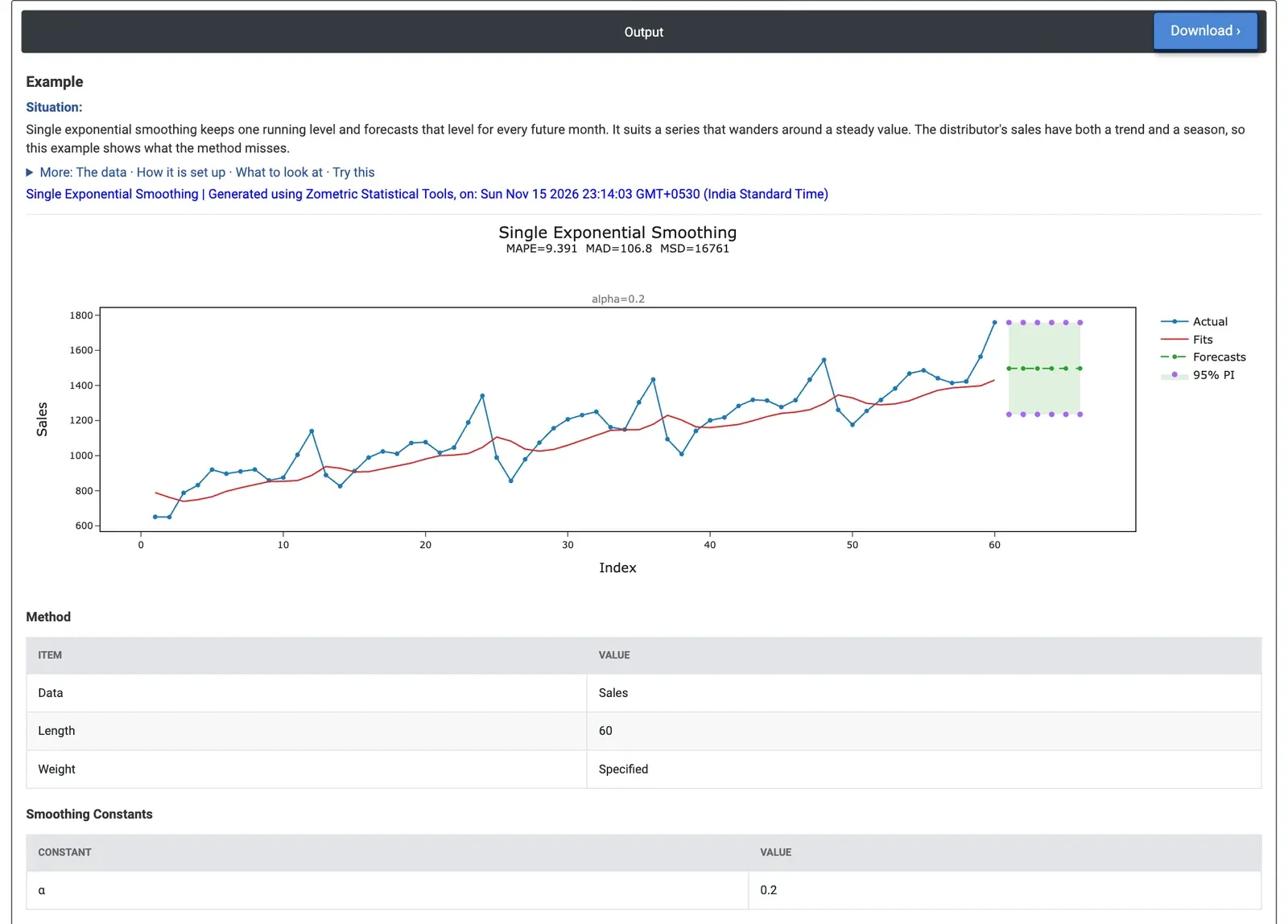
Figure 2 — The smoothed line lags behind the growing sales, and all six forecasts are the same, 1,496.7.
Worked Example
A consumer electronics distributor has 60 months of unit sales (January 2020 to December 2024). The sales analyst tries the simplest forecasting method first to see what it misses. The analyst selects Variable (Y) = Sales, enters Weight to use in smoothing (alpha) = 0.2, keeps Starting values = From the data and K = 6, and sets Number of forecasts = 6 for January to June 2025.
All six forecasts are the same: 1,496.7 units, with a 95% interval of 1,234.9 to 1,758.4. The method has no trend or season, so it cannot see that sales grow and that January and February are always weak. On the plot the smoothed line lags behind the rising data and cuts through the peaks and dips. MAPE is 9.4% (MAD 106.8 units), the weakest fit of the forecasting tools on this data: Winters' Method reaches 4.2% and Decomposition 2.2%.
When alpha is left blank, the optimal ARIMA weight is 1.43, above 1: the level overreacts to every month in an attempt to keep up with the growth. MAPE falls to 6.7%, but every month of 2025 is then forecast at 1,817, the level left by the December peak. Both results say the same thing for the decision: this series needs a method with a trend and a season. Single smoothing is the right tool only when the data have neither.