
3D Surface Plot
On this page
Purpose
The 3D Surface Plot draws a response Z as a surface over two variables X and Y, for example yield over temperature and reaction time. It shows where the response peaks or dips, how steeply it changes, and whether the best region is a sharp point or a broad plateau. Use it to explore results from a designed experiment or a process study with two settings, and to choose operating windows. The plot can be turned and zoomed with the mouse.
Key Capabilities
- Surface from grid data (every X/Y combination present) or from scattered X/Y points.
- Two interpolation methods for scattered data: Distance (inverse-distance weighting) or Akima's polynomial method.
- Automatic or user-set mesh size.
- Display elements you can combine: surface, wireframe, data points (symbols), project lines from each point to the base, and contour lines projected on the surface.
- Choice of colour scale, with a colour bar for Z.
Statistical Methods
The surface is an interpolation of the data, not a fitted model. When every X/Y combination is present (grid data, even or uneven spacing; replicates averaged), Akima's local cubic interpolation is applied through the grid along Y and then along X on a fine mesh (up to 201 points per axis). The surface passes through every measured point; the interpolation method, distance power and mesh settings have no effect on grid data.
For scattered data the response is estimated on an X × Y mesh (15 × 15 by default) spanning the range of the data. The Distance method uses Shepard's inverse-distance weighting, ẑ = Σ(zᵢ / dᵢᵖ) / Σ(1 / dᵢᵖ), where dᵢ is the distance from the mesh node to data point i and p is the Distance Power (default 2): higher powers give nearby points more weight. Estimates always stay within the range of the data. With Standardize X and Y ticked, X and Y are first scaled to −1 to 1, so a variable with a large numeric range does not dominate the distances. Akima's method fits smooth local polynomials over a triangulation of the points; it gives a smoother surface but can over- or undershoot the data, especially beyond the outermost points, where the Boundary z-value (or the lowest estimated Z) is used.
Because the surface only interpolates, small bumps can come from measurement scatter. To estimate an optimum with confidence, fit a response surface model (DOE response surface or regression) and use its fitted surface.
Input Fields & Options
Field | Description |
X Variable / Y Variable | Required. Numeric columns for the two horizontal axes. |
Z Variable (Response) | Required. Numeric response drawn as height and colour. |
Interpolation Method | Distance Method (default) or Akima's Polynomial Method. Ignored for grid data. |
Distance Power | Default 2.0. Distance method only; higher powers give nearby points more weight. |
Standardize X and Y data | Ticked by default. Distance method only. |
Boundary z-value | Optional. Akima's method only: Z used beyond the outermost data points; empty uses the lowest estimated Z. |
Automatic Mesh / X mesh size (columns) / Y mesh size (rows) | Automatic Mesh ticked by default (15 × 15). Untick to set the mesh sizes (2 to 500). Ignored for grid data. |
Surface / Wireframe / Symbols (data points) / Project lines / Project contours on surface | Display elements. Surface and Project contours on surface are ticked by default; at least one of Surface, Wireframe, Symbols or Project lines must be ticked. |
Color scale | Colour scale of the surface. Default Viridis. |
Title | Optional. Left empty (the default), the plot is titled “Surface Plot of Z vs Y, X” with the column names; otherwise the text entered. |
Data Options: Subset (optional) | Exclude matching rows (default) or Include only matching rows; Row numbers (e.g. 3,7,12-15) and/or a Condition (e.g. Temperature_C <= 200) select the rows. |
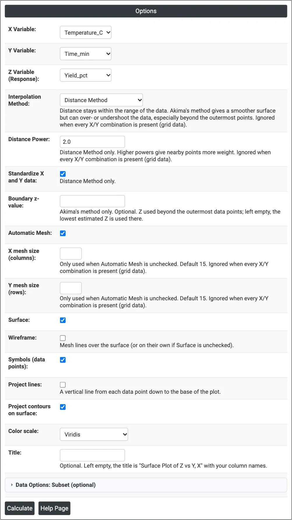
Figure 1 — Options for the example: Yield_pct over Temperature_C and Time_min, with the surface, data points and projected contours.
Output Descriptions
- Surface Plot of <Z> vs <Y>, <X> — the 3D surface with a colour bar for Z, plus the wireframe, data points, project lines and contours that are ticked; drag to rotate, scroll to zoom, hover to read values.
- PDF export via Download.
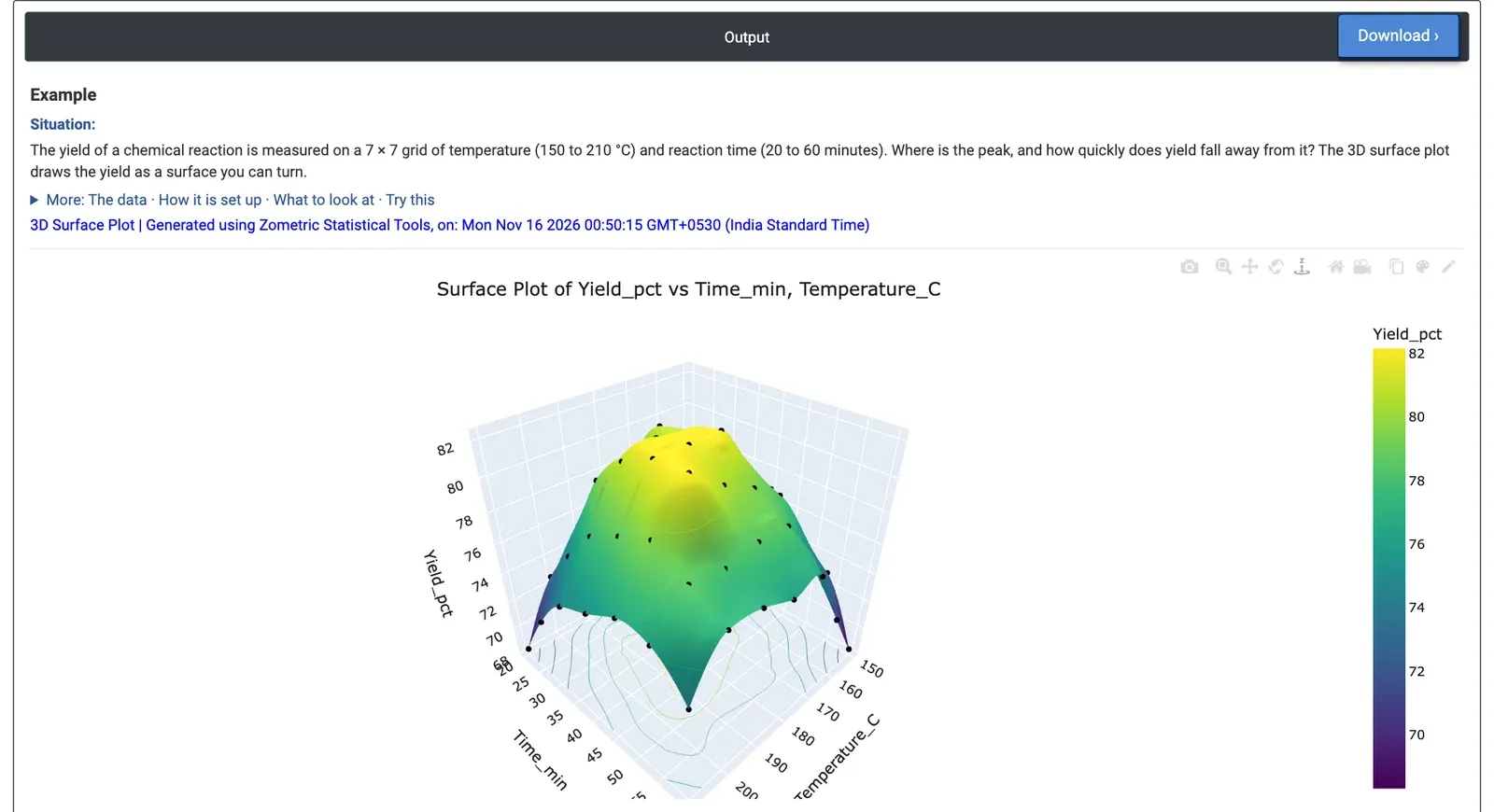
Figure 2 — Yield of a reaction over a 7 × 7 grid of temperature and time: a dome with a broad flat top, data points shown as dots.
Worked Example
A process engineer measures the yield of a chemical reaction on a 7 × 7 grid: temperatures from 150 to 210 °C in 10-degree steps and reaction times from 20 to 60 minutes, 49 runs in all. The questions are where yield peaks and how quickly it falls away. X Variable = Temperature_C, Y Variable = Time_min, Z Variable = Yield_pct, with Surface, Symbols and Project contours on surface ticked.
The surface is a dome: yield is highest in the middle of the grid and falls towards every edge. The top is flat. Five settings between 170 and 190 °C and 33.3 to 46.7 minutes all give 81.4% to 82.0%, the highest measured being 81.99% at 190 °C and 46.7 minutes; the interpolated surface peaks at about 82.2% near 188 °C and 42 minutes. The lowest yields are at two opposite corners: 68.30% at 150 °C and 60 minutes, and 68.32% at 210 °C and 20 minutes. Because the data form a complete grid, the surface passes through every measured point, and the small bumps on the top reflect measurement scatter rather than separate peaks.
For production this means there is a broad operating window around 170 to 190 °C and 35 to 45 minutes, so the team can choose the cheapest or fastest setting inside it without losing yield. Moving away from it costs more yield at the corners where high temperature meets short time, or low temperature meets long time. The Contour Plot on the same columns shows the same window as a flat map.