
Symmetry Plot
On this page
Purpose
The Symmetry Plot checks whether a set of measurements is symmetric about its median. It pairs the values from the two ends of the sorted data and compares how far each lies below and above the median. Symmetric data fall along a 45-degree line; a long upper or lower tail pulls the points off it. Use it before methods that assume a symmetric, bell-shaped distribution (t-tests, normal capability, control limits) and to see which tail causes any skewness.
Key Capabilities
- One point per pair of observations equally far in rank from the median.
- Dashed symmetry line through the origin at 45 degrees, with both axes on the same range.
- Shows which tail is longer and which observations cause it, not just whether the data are skewed.
- Works with any numeric column of at least 4 values; rows can be excluded by row number or condition.
Statistical Methods
The non-blank numeric values are sorted, x₍₁₎ ≤ … ≤ x₍ₙ₎, and the median M is found. The values below the median are paired, from the closest to the furthest, with the values above it: the largest value below the median with the smallest value above it, and so on, out to the smallest value with the largest. For odd n the median value itself is left out; for even n the median is the average of the two middle values, which form the first pair.
For pair i, the plot shows the distance below the median, M − x₍ₖ₊₁₋ᵢ₎, on the horizontal axis and the distance above the median, x₍ₙ₋ₖ₊ᵢ₎ − M, on the vertical axis, where k = ⌊n/2⌋. If the distribution is symmetric, each pair is about equally far from the median and the points lie near the line y = x. Points that rise above the line mean the upper values spread further than the lower ones: a long upper tail, or right skew. Points below the line mean a long lower tail, or left skew. Points near the origin come from the centre of the data and points far out from the tails, so deviations at the right end of the plot concern the most extreme values.
The plot gives no test statistic. Some scatter about the line is normal, especially for the outer points; judge the overall trend. A normal probability plot or a normality test complements it.
Input Fields & Options
Field | Description |
Variable | Required. Numeric column to check (at least 4 values). |
Title | Title of the plot. Default “Symmetry Plot”. |
Data Options: Subset (optional) | Exclude matching rows (default) or Include only matching rows; Row numbers (e.g. 3,7,12-15) and/or a Condition (e.g. Batch_Type == "Standard") select the rows. |
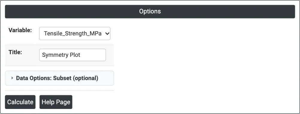
Figure 1 — Options for the example: Variable = Tensile_Strength_MPa.
Output Descriptions
- Symmetry Plot — distance below the median (horizontal) against distance above the median (vertical) for each pair, with the dashed red symmetry line.
- PDF export via Download.
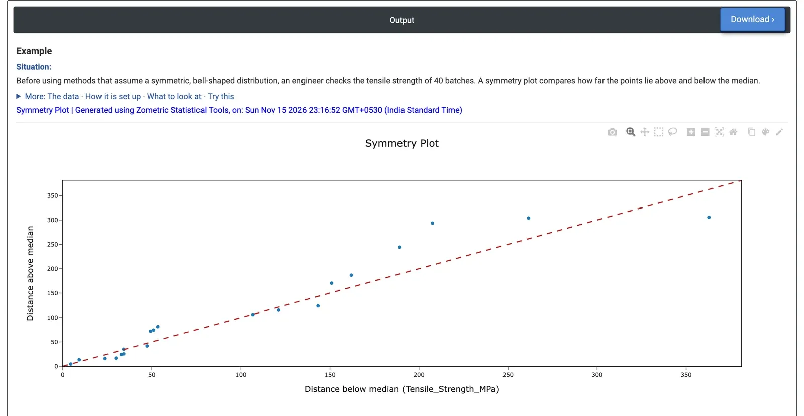
Figure 2 — Symmetry plot of the tensile strength of 40 batches: 20 pairs close to the line, with the outermost pair below it.
Worked Example
Before using control limits and capability indices that assume a bell-shaped distribution, a quality engineer checks whether the tensile strength of 40 material batches is symmetric. Variable = Tensile_Strength_MPa.
The median is 1185.4 MPa, and the 40 values give 20 pairs. Most points lie close to the dashed line, and 10 of the 20 pairs lie above it, the rest on or below it: there is no consistent tail. The outermost point, at the right of the plot, lies clearly below the line: the weakest batch (822.6 MPa) is 362.8 MPa below the median, while the strongest (1490.9 MPa) is only 305.5 MPa above it. One low batch makes the lower tail a little longer than the upper one.
Computed from the same data, the skewness is 0.06 and a Shapiro-Wilk normality test gives p = 0.45, so the data are close enough to symmetric for normal-based methods. The engineer would still look up the 822.6 MPa batch to check whether it had a special cause, because a single extreme value is what drives the only departure from the line. Running the same plot for Density_gcc (skewness −0.25) puts 13 of the 20 pairs on or below the line, a mild long lower tail.