
Trend Analysis
On this page
Purpose
Trend Analysis fits a trend line or curve to a time series and extends it to forecast future periods. It answers questions such as “how fast is demand growing each month?” or “where will this wear measurement be in six months if the trend continues?”. Use it for a series with a long-term trend and no strong seasonal pattern, or as a first look before a seasonal method such as Decomposition or Winters' Method.
Key Capabilities
- Four trend models: Linear, Quadratic, Exponential Growth and S-Curve.
- Fitted trend equation, forecasts for any number of periods, and MAPE, MAD and MSD accuracy measures.
- Time axis labelled from a date or stamp column, or by row number.
- Forecast origin to forecast from an earlier row and compare with known data.
- Weighted trend analysis: blend estimates from a previous fit with the new ones.
- Optional results table (trend and detrended value for each period) and four-in-one residual plots.
Statistical Methods
The time index is t = 1, 2, … n (the row order). Linear fits Yt = b₀ + b₁·t and Quadratic fits Yt = b₀ + b₁·t + b₂·t², both by least squares. Exponential Growth fits Yt = b₀·b₁ᵗ by a least-squares line on the logarithm of the data, so b₁ is the growth factor per period (1.01 = 1% a period). S-Curve fits the Pearl-Reed logistic curve Yt = 10ᵃ / (b₀ + b₁·b₂ᵗ) by non-linear least squares, which levels off at an upper limit. Exponential Growth and S-Curve need all values above zero.
Fits are the trend values, and forecasts extend the equation to t = n + 1, n + 2 … (or from the forecast origin, using a trend fitted to the data up to that row). No prediction limits are given. Accuracy: MAPE = mean |error / data| × 100, MAD = mean |error| and MSD = mean error², where error = data − trend; the detrended values in the results table are data − trend (data / trend for Exponential Growth and S-Curve).
Weighted trend analysis: enter the estimates of a previous fit as Prior parameter values (b₀ b₁ …, in output order). Each blended estimate is w × new + (1 − w) × prior, with w = 0.2 by default, so a new period of data updates an established trend gently instead of replacing it. The series must have no gaps and at least 4 values.
Input Fields & Options
Field | Description |
Variable (Y) | Required. The numeric series, in time order. |
Time/stamp column | Optional. Labels the time axis (e.g. a month column); row order (Index) is used if left blank. It does not change the fit. |
Model type | Linear (default), Quadratic, Exponential Growth or S-Curve. |
Number of forecasts | Default 0 (none), up to 1000. |
Forecast origin (row) | Optional, active when forecasts are requested. Forecasts start after this row, using the data up to it; blank = end of the series. |
Prior parameter values | Optional. Estimates from a previous fit, in output order (b0 b1 …), for a weighted trend analysis. |
Weights for blending priors with new estimates | Active when prior values are entered. Between 0 and 1, one per estimate; blank = 0.2 each. Blended = w × new + (1 − w) × prior. |
Results to display | Summary table (default) or Summary table and results table. |
Residual plots (four in one) | Unticked by default. Normal probability plot, residuals versus fits, histogram and residuals versus order. |
Title | Title of the output. Default Trend Analysis. |
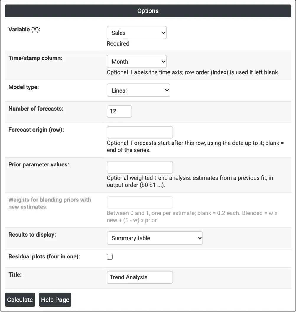
Figure 1 — Linear trend of monthly Sales, labelled by Month, with 12 forecasts.
Output Descriptions
- Trend Analysis (graph) — actual data, fitted trend and forecasts, with MAPE, MAD and MSD in the title.
- Method — data column, length and model type (plus weighted analysis and forecast origin when used).
- Fitted Trend Equation — the equation with its estimates.
- Weighted Estimates — when priors are entered: Parameter, Prior, New, Weight and Blended.
- Accuracy Measures — MAPE, MAD and MSD.
- Forecasts — period and forecast.
- Results — when chosen: Period, data, Trend and Detrend for each period.
- Residual Plots — when ticked.
- PDF export via Download.
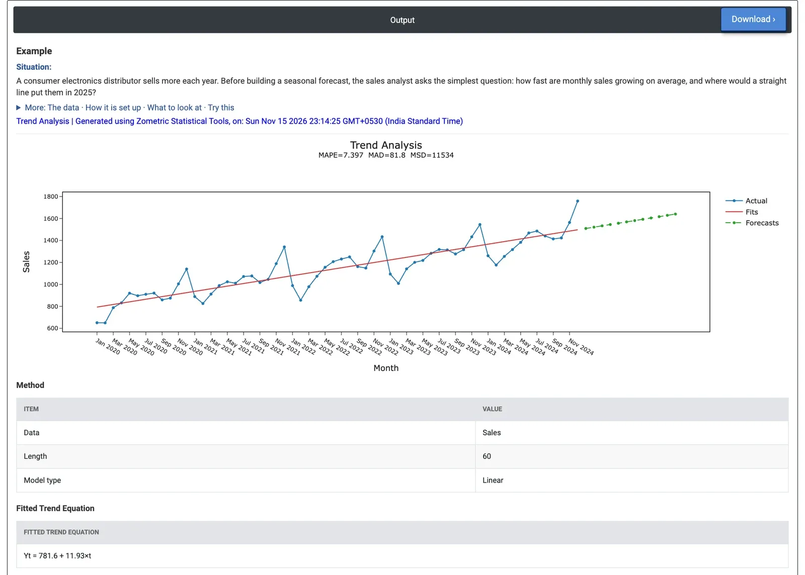
Figure 2 — A straight line through 60 months of sales: about 12 more units each month.
Worked Example
A consumer electronics distributor sells more each year. Before building a seasonal forecast, the sales analyst asks the simplest question: how fast are monthly sales growing on average, and where would a straight line put them in 2025? The analyst has 60 months of unit sales (January 2020 to December 2024) and selects Variable (Y) = Sales, Time/stamp column = Month, Model type = Linear and Number of forecasts = 12.
The fitted trend is Yt = 781.6 + 11.93×t: sales grow by about 12 units a month, or about 143 a year. The line forecasts 1,509 for January 2025 (period 61) rising to 1,641 for December 2025 (period 72). MAPE is 7.4% (MAD 81.8 units): the months sit on average 7.4% away from the line, mostly because of the season. Every December is 191 to 273 units above the line (December 2024: 1,759 against 1,497) and every February 123 to 236 units below it.
For the decision this means the line gives a sound growth rate but will under-forecast the year-end peak and over-forecast the early-year dip. The Quadratic model gives a curve term of only 0.00093×t² and the same MAPE (7.4%), so the growth is close to a straight line; Exponential Growth (1.08% a month) fits slightly worse, with MAPE 7.6%. For monthly forecasts that follow the season, use Decomposition (MAPE 2.2%) or Winters' Method on the same data.