
2-Sample Poisson Rate Test
On this page
Purpose
The 2-Sample Poisson Rate Test compares the rates at which events occur in two groups, such as stoppages per shift on day and night shifts, defects per unit from two lines, or complaints per month before and after a change. It estimates the difference between the two rates with a confidence interval and tests whether it differs from zero or from another hypothesized difference. Use it for counts of independent events over a known amount of exposure; for pass/fail results use the 2 Proportions test.
Key Capabilities
- Data as summarized counts, as two columns of counts, or as one column of counts with a column of sample IDs.
- Exact test (conditional binomial) and normal approximation side by side when the hypothesized difference is 0.
- Variance of the difference from the separate rates or from the pooled rate.
- Two-sided or one-sided alternatives, with a confidence interval or a one-sided bound for the difference.
- Different observation lengths for the two samples, e.g. 8-hour and 12-hour shifts.
Statistical Methods
For sample i with Nᵢ units, each observed over a length tᵢ (Observation length), the exposure is Tᵢ = Nᵢ·tᵢ and, with Xᵢ events in total, the rate is λ̂ᵢ = Xᵢ / Tᵢ. The estimated difference is D = λ̂₁ − λ̂₂, Sample 1 minus Sample 2. With two-column or stacked data, Nᵢ is the number of non-blank counts in the sample and Xᵢ their sum.
Normal approximation: z = (D − D₀) / SE, where D₀ is the hypothesized difference. With Estimate the rates separately, SE = √(λ̂₁ / T₁ + λ̂₂ / T₂); with Use the pooled estimate of the rates, SE = √[λ̂ₚ(1 / T₁ + 1 / T₂)] with λ̂ₚ = (X₁ + X₂) / (T₁ + T₂). When the two exposures are equal, the two methods give the same SE. The p-value comes from the standard normal distribution, and the confidence interval for the difference is D ± z·SE (or a one-sided bound).
Exact test, given only when D₀ = 0: if the rates are equal, the count X₁ out of the total X₁ + X₂ follows a binomial distribution with probability T₁ / (T₁ + T₂). The one-sided p-values are the binomial tails, and the two-sided p-value is twice the smaller tail. The exact test is preferred when the counts are small. Both methods assume that events occur independently at a constant rate within each group.
Input Fields & Options
Field | Description |
Data | Summarized data (default), Each sample is in its own column, or Both samples are in one column. |
Sample 1 / Sample 2 | With Each sample is in its own column: the two columns of counts. |
Samples / Sample IDs | With Both samples are in one column: the column of counts and the column naming the sample of each row (exactly two distinct values; the first one found is Sample 1). |
Sample 1 sample size / Sample 1 total occurrences / Sample 2 sample size / Sample 2 total occurrences | With Summarized data: the number of units and the total number of events in each sample. |
Hypothesized difference | Default 0. The value of λ₁ − λ₂ under the null hypothesis; the exact test is given only for 0. |
Confidence level | Default 95; 75 to 100. |
Alternative hypothesis | Difference ≠ hypothesized difference (default), Difference < hypothesized difference or Difference > hypothesized difference. |
Test method | Estimate the rates separately (default) or Use the pooled estimate of the rates, for the normal approximation. |
Observation length (Sample 1) / Observation length (Sample 2) | Default 1. The exposure of each unit; Sample 2 uses the Sample 1 length when left blank. |
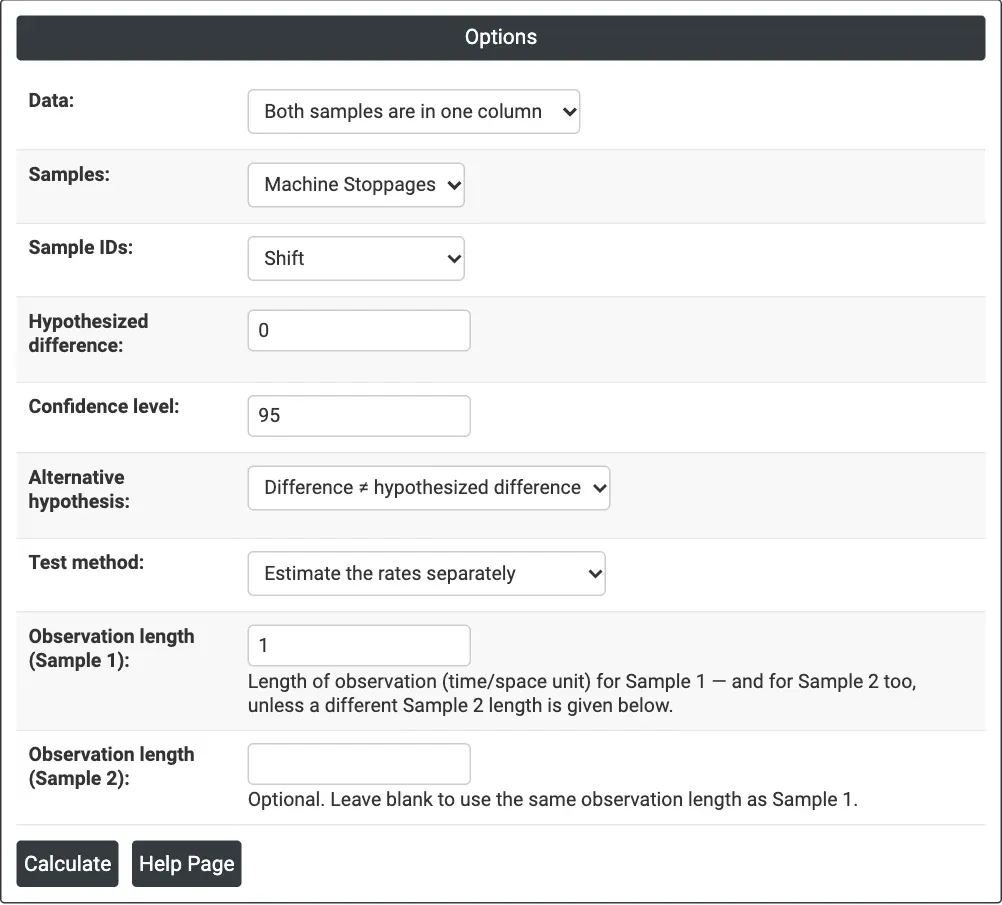
Figure 1 — Options for the example: Machine Stoppages stacked in one column with Shift as the sample IDs, two-sided, rates estimated separately.
Output Descriptions
- Method — which sample is λ₁ and which is λ₂, and the difference λ₁ − λ₂.
- Descriptive Statistics — Sample, N, Total Occurrences and Sample Rate for each sample.
- Estimation for Difference — the Estimated Difference and its confidence interval (or upper or lower bound).
- Test — the null and alternative hypotheses, and a table with the Z-Value and P-Value for the Exact and Normal approximation methods, with a note when the pooled estimate is used.
- PDF export via Download.
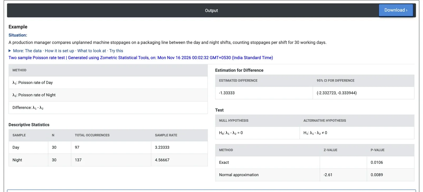
Figure 2 — Day shifts average 3.233 stoppages and night shifts 4.567; the 95% CI for the difference, −2.333 to −0.334, excludes 0 (exact p = 0.0106).
Worked Example
A production manager compares unplanned machine stoppages on a packaging line between the day and night shifts, counting the stoppages in each shift over 30 working days. Data = Both samples are in one column, Samples = Machine Stoppages, Sample IDs = Shift, Hypothesized difference = 0, Confidence level = 95, two-sided, Test method = Estimate the rates separately, Observation length = 1 (one shift).
The day shifts had 97 stoppages in 30 shifts, a rate of 3.233 per shift, and the night shifts 137 in 30 shifts, 4.567 per shift. The estimated difference, Day minus Night, is −1.333 stoppages per shift, with a 95% CI of −2.333 to −0.334: the interval excludes 0. The exact test gives p = 0.0106 and the normal approximation z = −2.61, p = 0.0089. The night shift has more stoppages, about 40% more than the day shift.
Because both samples cover 30 shifts, Use the pooled estimate of the rates gives the same z and p-value here. If the manager had expected the night shift to be worse before collecting the data, Difference < hypothesized difference gives p = 0.0053 (exact) and a 95% upper bound of −0.495 for the difference. The next step is to find out what differs at night, for example staffing, changeovers or material, before the extra stoppages cost more output.