
Winters' Method
On this page
Purpose
Winters' Method (Holt-Winters, or triple exponential smoothing) smooths a time series with three running components: a level, a trend and a seasonal index for each period of the season. Its forecasts grow with the trend and repeat the seasonal pattern. Use it for monthly, quarterly or shift-pattern data with both a trend and a season, for example to forecast demand, energy use or workload for the coming year, when the pattern changes slowly over time.
Key Capabilities
- Multiplicative method (the seasonal swing grows with the level) or additive method (the swing stays the same size).
- Separate weights for level (alpha), trend (gamma) and season (delta), 0.2 each by default.
- Starting values from the data or values you enter, including one seasonal index per period.
- Forecasts with prediction limits that widen with each period ahead, from the end of the series or from an earlier row to test the method against known data.
- MAPE, MAD and MSD accuracy measures, a plot of the data, fits and forecasts, an optional results table and four-in-one residual plots.
Statistical Methods
For the multiplicative method, with seasonal length p, the components are updated each period: level Lₜ = α·(yₜ / Sₜ₋ₚ) + (1 − α)·(Lₜ₋₁ + Tₜ₋₁); trend Tₜ = γ·(Lₜ − Lₜ₋₁) + (1 − γ)·Tₜ₋₁; seasonal index Sₜ = δ·(yₜ / Lₜ) + (1 − δ)·Sₜ₋ₚ. The fit for period t is (Lₜ₋₁ + Tₜ₋₁)·Sₜ₋ₚ, and the forecast m periods after the origin is (L + m·T) × the latest index for that period of the season. The additive method subtracts and adds the seasonal term instead of dividing and multiplying.
Starting values from the data: the initial level and trend are the intercept and slope of a least-squares line through the first season. For the multiplicative method each initial index is the average of that period over all the data divided by the overall average; for the additive method it is the average, for that period, of the residuals from a straight line fitted to the whole series. The weights are used as entered (blank counts as 0.2); they are not optimised. With Starting values = User-specified you enter the initial level, trend and p seasonal indices.
The prediction limits are forecast ± z × dₘ × MAD, where z is the normal quantile for the confidence level, MAD is the mean absolute error of the fits and dₘ grows with the number of periods ahead m (computed from the largest of the three weights). Accuracy: MAPE = mean |error / data| × 100, MAD = mean |error|, MSD = mean error². The series needs at least two full seasons and no gaps; the multiplicative method needs all values above zero.
Input Fields & Options
Field | Description |
Variable (Y) | Required. The numeric series, in time order. |
Seasonal length | Required, at least 2. Periods per season, e.g. 12 for monthly data with a yearly pattern. |
Method type | Multiplicative (default) or Additive. |
First observation is in seasonal period | Default 1. The position of the first row in the season, e.g. 6 when the season starts in January and the data start in June. |
Level weight (alpha) / Trend weight (gamma) / Seasonal weight (delta) | 0.0001 to 1, default 0.2 each. Larger values let that component react faster to recent data. |
Starting values | From the data (default) or User-specified. |
Initial level / Initial trend / Initial seasonal indices | Used when Starting values is User-specified; all three are then required. Seasonal indices: comma or space-separated, one per period of the season (Seasonal length values). |
Number of forecasts | Default 0 (none), up to 1000. |
Confidence level (%) for forecast interval | Default 95. Active when forecasts are requested. |
Forecast origin (row) | Optional, active when forecasts are requested. Forecasts start after this row, using the data up to it; blank = end of the series. |
Results to display | Summary table (default) or Summary table and results table. |
Residual plots (four in one) | Unticked by default. |
Title | Title of the output. Default Winters' Method. |
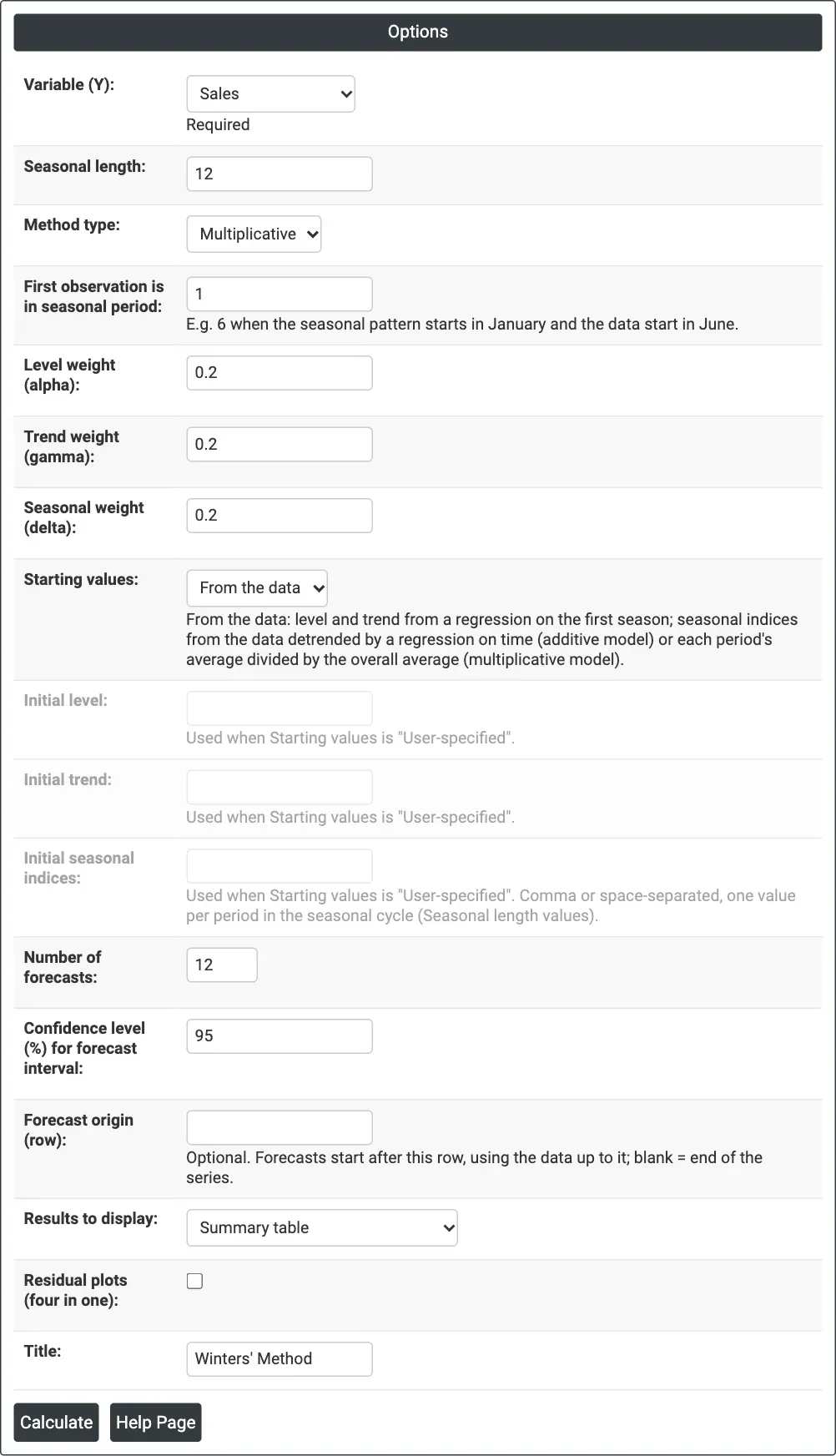
Figure 1 — Multiplicative Winters' Method on monthly Sales, seasonal length 12, weights 0.2 each and 12 forecasts.
Output Descriptions
- Winters' Method (graph) — actual data, fits, forecasts and the prediction band, with MAPE, MAD and MSD in the title and the three weights above the plot.
- Method — model type, data column and length (plus the first seasonal period and forecast origin when set).
- Smoothing Constants — α (level), γ (trend) and δ (seasonal).
- Accuracy Measures — MAPE, MAD and MSD.
- Forecasts — period, forecast, lower and upper limits.
- Results — when chosen: Period, data, Season, Level, Trend, Seasonal, Predict and Error for each period.
- Residual Plots — when ticked.
- PDF export via Download.
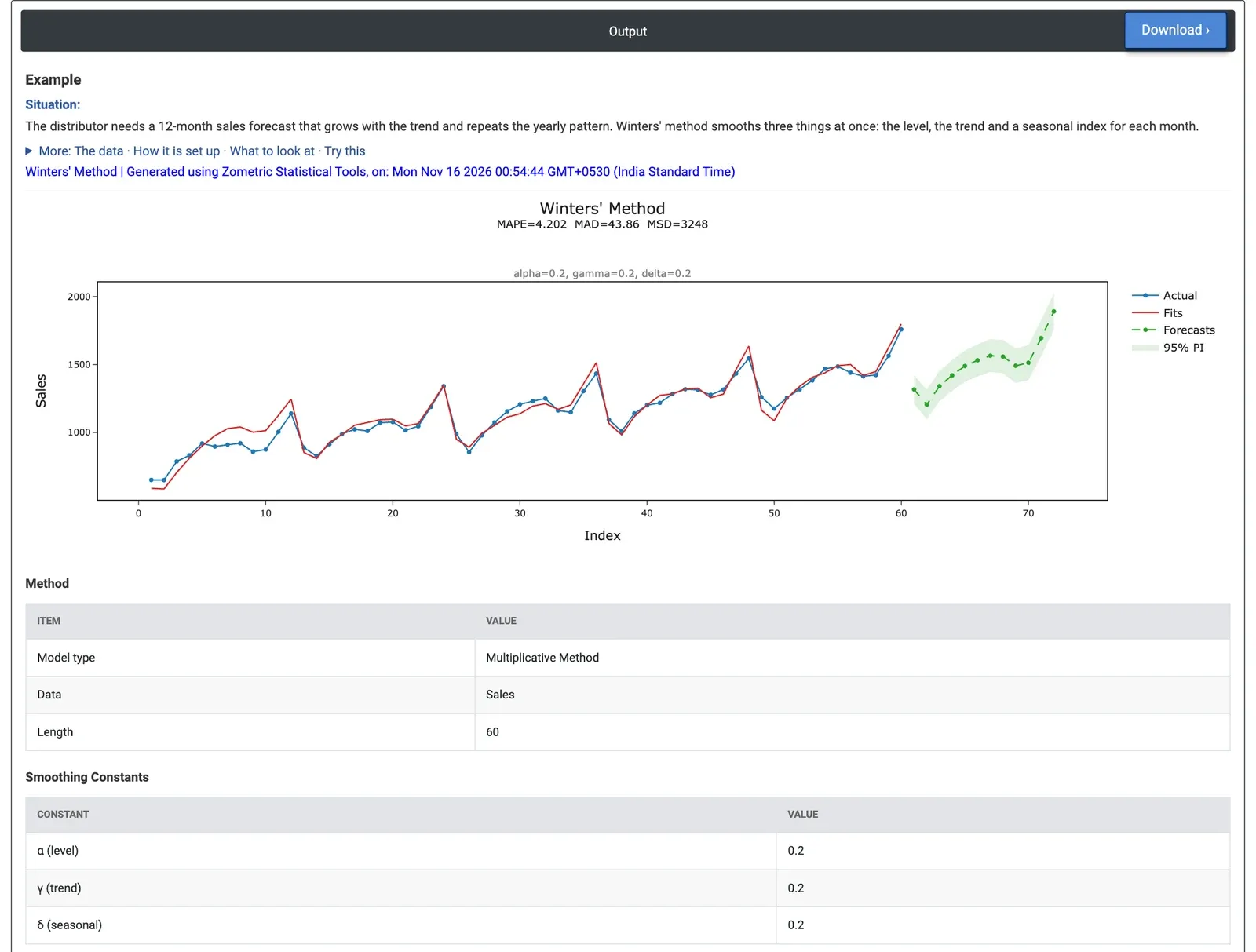
Figure 2 — The 2025 forecasts repeat the yearly shape on a higher level, from a low of 1,205 in February to 1,891 in December.
Worked Example
A consumer electronics distributor needs a 12-month sales forecast for 2025 that grows with the trend and repeats the yearly pattern of weak early months and a December peak. The analyst has 60 months of unit sales (January 2020 to December 2024). The analyst selects Variable (Y) = Sales, Seasonal length = 12 and Method type = Multiplicative, keeps the three weights at 0.2, and sets Number of forecasts = 12.
The forecasts run from 1,317 in January 2025, down to the low point of 1,205 in February, up to 1,891 in December, with 95% limits of 1,756 to 2,026 for December. The intervals widen from about ±107 units in January to ±135 in December. MAPE is 4.2% (MAD 43.9 units), far better than the smoothing methods without a season (8.3% to 9.4%). December 2025 at 1,891 compares with 1,759 in December 2024: about 7.5% growth.
To test the method, Forecast origin (row) = 48 forecasts 2024 from the data up to December 2023. Eleven of the twelve actual months fall inside the 95% limits (February 2024, at 1,176, is one unit above its upper limit), and the forecasts miss by 4.9% on average; but every month is under-forecast, because growth picked up in 2024. With Method type = Additive the MAPE drops to 3.7%, so a fixed number of units per month fits this season slightly better than a percentage. Weights of 0.4, 0.1 and 0.3 give 3.8%, no better than the defaults.