
Binary Fitted Line Plot
Binary Fitted Line Plot models the probability of a pass/fail or yes/no outcome against one continuous predictor, using raw binary rows or event/trial counts and a logit, probit or complementary log-log link. Output includes the regression equation, deviance ANOVA, Deviance R-Sq, AIC, area under the ROC curve, coefficients, odds ratios (logit), the fitted curve and unusual observations.
Last reviewed
Key takeaway
A binary fitted line plot fits a logistic (or probit) regression of a yes/no outcome on one continuous predictor and draws the S-shaped probability curve, showing how far a setting must move before the event becomes likely.
On this page
Purpose
Binary Fitted Line Plot models how the probability of a yes/no outcome changes with one continuous predictor, and draws the fitted S-shaped curve over the data. Use it when the result is pass/fail, defective/good or caked/not caked, and you want to know how far a setting such as temperature, humidity or dose must move before the event becomes likely.
Key Capabilities
- Accepts raw data (one row per unit with a yes/no column) or summarised data (number of events and number of trials per row).
- Logit, probit or complementary log-log link.
- Regression equation, deviance ANOVA table, model summary, coefficients with confidence intervals and, for the logit link, the odds ratio for any increment of the predictor.
- Plot of the fitted probability curve with optional observed proportions and confidence band.
- Table of unusual observations (large residuals or unusual predictor values) and optional residual plots.
- Optional frequency column for data with repeated rows.
Statistical Methods
The tool fits a binary logistic regression with one predictor as a generalised linear model with a binomial distribution, by maximum likelihood (iteratively reweighted least squares). With the logit link, P(event) = exp(b₀ + b₁x) / (1 + exp(b₀ + b₁x)); with probit, P = Φ(b₀ + b₁x); with complementary log-log, P = 1 − exp(−exp(b₀ + b₁x)). In raw-data format, rows whose response equals the Event value count as events and all others as non-events.
The ANOVA table tests the predictor by the drop in deviance: χ² = null deviance − residual deviance, with 1 degree of freedom. Deviance R-Sq is the share of the null deviance explained. The coefficient table gives Wald z-values and confidence intervals b ± z·SE; the odds ratio for an increment Δ is exp(b₁·Δ), with interval exp(Δ × the limits of b₁). Area Under ROC Curve is the chance that a randomly chosen event has a higher fitted probability than a randomly chosen non-event (0.5 = no discrimination, 1 = perfect).
The confidence band around the curve uses the standard error of the linear predictor, transformed back to the probability scale. In the unusual observations table, a standardised residual beyond ±2 is flagged R and a leverage above 3p/n is flagged X. With raw data the observed proportions on the plot are the event rates within up to 10 groups of equal size along the predictor.
Input Fields & Options
Field | Description |
Data format | Binary response (one row per observation, default) or Event/Trial (one row per setting with a count of events and a count of trials). |
Response / Event value | Binary response format: the column holding the outcome, and the value in it that counts as the event (e.g. Yes, Fail, 1). |
Number of events / Number of trials | Event/Trial format: the columns with the count of events and the number of units tested on each row. |
Event name | Optional label for the event, used in the equation and plot axis, e.g. Caked. Blank: the Event value (Binary response format) or the name of the events column (Event/Trial format). |
Predictor (continuous) | Numeric predictor. Required. |
Link function | Logit (default), Probit or Complementary log-log. |
Confidence level | Default 95. |
Type of confidence interval | Two-sided (default), Lower bound or Upper bound; applies to coefficients, odds ratios and the curve band. |
Frequency (optional) | Column with the number of times each row occurs. |
Increment for odds ratio | Change in the predictor for which the odds ratio is reported. Default 1. Logit link only. |
Display observed proportions / Display confidence interval | Add the observed event proportions and the confidence band to the plot. Off by default. |
Residuals for plots | Regular or Deviance residuals for the residual plots. |
Histogram of residuals / Normal probability plot of residuals / Residuals versus order / Three in one | Residual plots; Three in one draws all three together. |
Residuals versus the variables | Plot the residuals against a chosen column. |
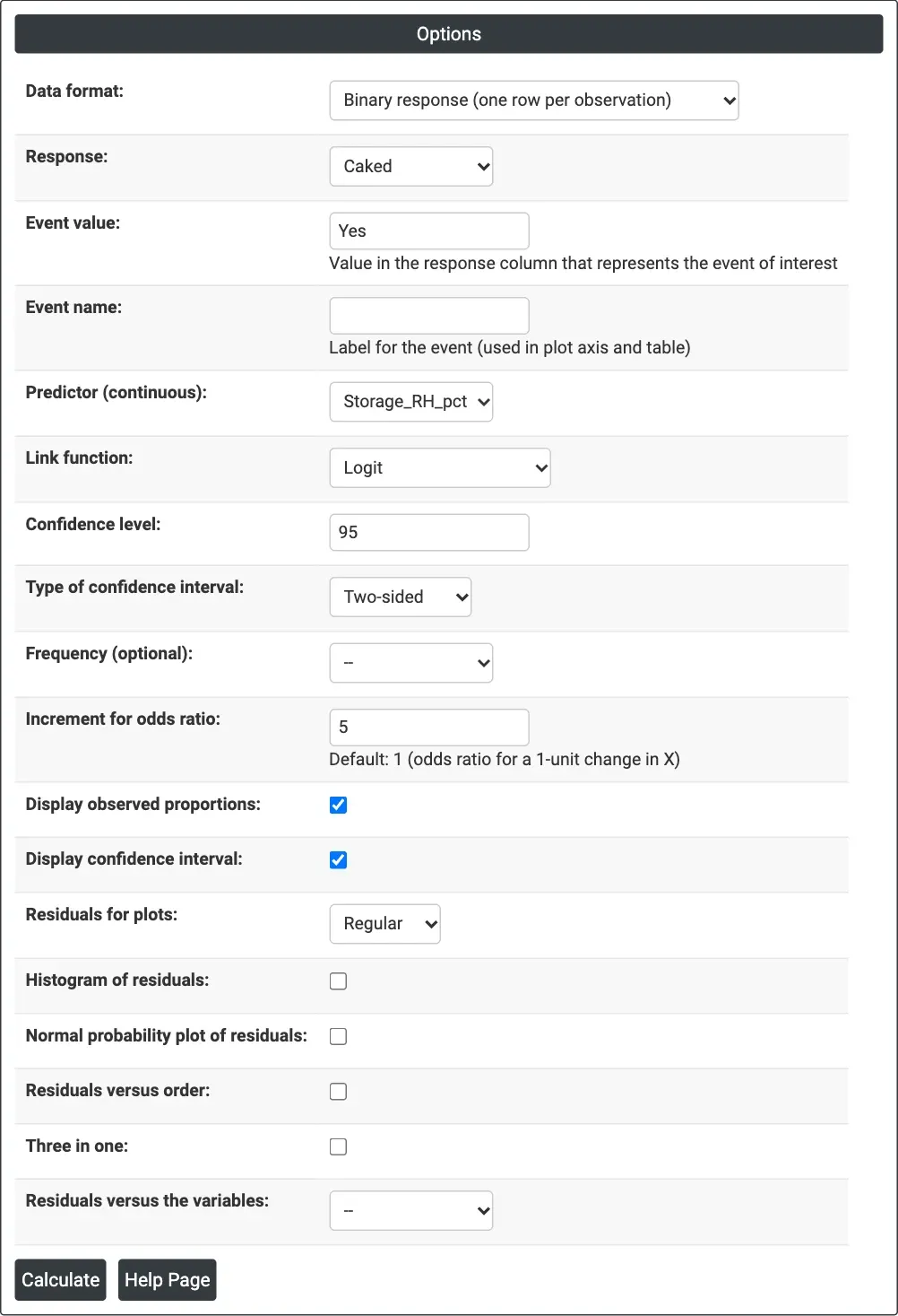
Figure 1 — Options for the bag caking example: Caked as the response with event Yes, Storage_RH_pct as the predictor, logit link, odds ratio for a 5-point increase in humidity.
Output Descriptions
- Regression Equation — the fitted probability of the event as a function of the predictor.
- Analysis of Variance — deviance test of the predictor (Adj Dev, Chi-Square, P-Value), with error and total deviance.
- Model Summary — Deviance R-Sq, Deviance R-Sq(adj), AIC, AICc, BIC and Area Under ROC Curve.
- Coefficients — Coef, SE Coef, Z-Value, P-Value and confidence limits for the constant and the predictor.
- Odds Ratios for Continuous Predictors (or Odds Ratios (Increment=Δ)) — logit link only.
- Binary Fitted Line Plot — fitted probability curve, with observed proportions and the confidence band if ticked.
- Fits and Diagnostics for Unusual Observations — rows flagged R (large residual) or X (unusual X).
- Residual plots, if selected.
- PDF export via Download.
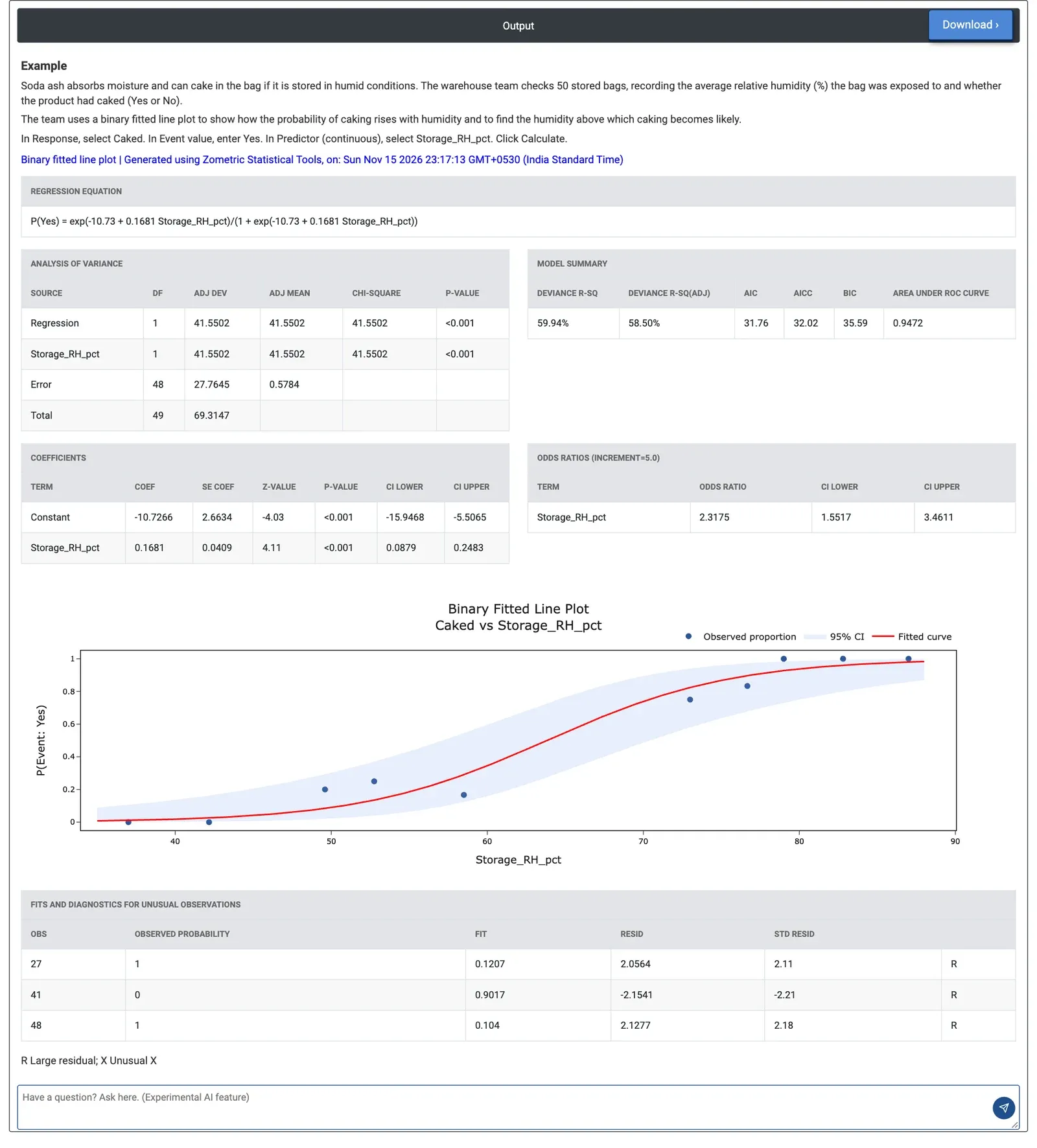
Figure 2 — Binary fitted line plot of the chance of caking against storage humidity: the curve passes 50% at about 64% RH.
Worked Example
Soda ash can cake in the bag when stored in humid conditions. A warehouse team checks 50 stored bags, noting the average relative humidity each bag was exposed to (Storage_RH_pct, 35 to 88%) and whether the product had caked (Caked: 25 Yes, 25 No). They select Caked as the response with Event value Yes, Storage_RH_pct as the predictor, keep the logit link, set the odds ratio increment to 5 and tick both display options.
Humidity has a clear effect: the deviance chi-square is 41.55 with p < 0.001, Deviance R-Sq is 59.94% and the area under the ROC curve is 0.9472, so humidity separates caked from sound bags well. The equation is P(Yes) = exp(−10.73 + 0.1681 RH) / (1 + exp(−10.73 + 0.1681 RH)). Each 5-point rise in humidity multiplies the odds of caking by 2.32 (95% CI 1.55 to 3.46). From the equation, the chance of caking is about 19% at 55% RH, 50% at 63.8% RH and 74% at 70% RH.
Three bags are flagged as unusual: two caked at low fitted probabilities (0.12 and 0.10) and one stayed sound at 0.90; worth checking for other causes such as damaged liners. To keep the caking risk below about 10%, the curve points to storage below roughly 51% RH. Switching to the probit link gives almost the same fit (Deviance R-Sq 60.50%).
Frequently asked questions
What is a binary fitted line plot?
A binary fitted line plot models how the probability of a yes/no outcome, such as pass/fail or caked/not caked, changes with one continuous predictor, and draws the fitted S-shaped curve over the data. It is a binary logistic regression with one predictor, fitted by maximum likelihood, with a logit, probit or complementary log-log link.
How do you interpret the odds ratio in a binary fitted line plot?
With the logit link, the odds ratio for an increment of the predictor is exp(b1 x increment). It is the factor by which the odds of the event are multiplied for that change. In the example, each 5-point rise in storage humidity multiplied the odds of caking by 2.32, with a 95% confidence interval of 1.55 to 3.46.
How do you know if the predictor has a significant effect?
The ANOVA table tests the predictor by the drop in deviance, a chi-square with 1 degree of freedom; a small p-value means a clear effect. Deviance R-Sq shows the share of null deviance explained, and the area under the ROC curve shows discrimination, where 0.5 means none and 1 means perfect.
How do you make a binary fitted line plot in Zometric Statistical Software?
Choose the data format: a binary response column with an Event value, or columns for number of events and trials. Select the continuous predictor and a link function (logit by default), set the confidence level and the odds ratio increment, and optionally display observed proportions and the confidence band. The output gives the equation, tables and plot.