
Capability Sixpack (Non-normal)
The Nonnormal Capability Sixpack suits data that are not normal, such as surface roughness, particle size or time-to-failure. You choose a distribution, such as Weibull, Lognormal or Gamma, fitted by maximum likelihood. The report shows I and MR charts with Nelson rules on the raw scale, a fitted histogram, a probability plot, the last 25 observations, and Pp, PPL, PPU and Ppk by the z-score method.
Last reviewed
Key takeaway
The nonnormal capability sixpack is a multi-panel report for skewed or bounded data that combines I-MR control charts, a fitted-distribution histogram and a probability plot with Pp and Ppk from a chosen nonnormal distribution.
On this page
Purpose
The Nonnormal Capability Sixpack gives the same at-a-glance, multi-panel process-health report as the app's Normal capability sixpack, but built for processes whose data does not follow a Normal distribution (bounded, skewed measurements such as surface roughness, particle size, or time-to-failure data). It combines a run chart, a fitted-distribution histogram and a probability plot into one report instead of forcing a Normal-distribution model onto data it doesn't fit.
Key Capabilities
- Fits any of the app's supported nonnormal distributions (e.g. Weibull, Lognormal, Gamma) by explicit user choice, rather than assuming Normality.
- Combines an I Chart and MR Chart (run-chart panel) with a fitted-distribution histogram and a probability plot in one 4-panel report.
- Full Nelson's-rules special-cause detection (8 configurable rules) on the run-chart panel, consistent with every other control chart in the app.
- Optional Factor column and “Compare selected columns as separate groups” mode.
- Configurable K-sigma tolerance and moving-range-based sigma estimation for the run-chart control limits.
Statistical Methods
The run-chart panel (I Chart and MR Chart) uses the app's standard Individuals/Moving-Range control chart machinery with Western-Electric/Nelson rule checks: the center line is the process mean, moving ranges are computed with the specified span (default 2), and control limits derive from MRbar/d2 (or median-moving-range) — independent of the distribution fitted for the capability panels, so the run chart always assesses statistical control on the raw, untransformed scale.
The histogram panel fits the user-selected candidate distribution to the sample via maximum-likelihood estimation and overlays its probability density function on the sample histogram, with LSL/USL reference lines where supplied.
The probability-plot panel transforms the sorted sample and the fitted distribution's plotting positions onto distribution-specific probability paper, so a well-fitting distribution appears as points falling close to a straight reference line — a visual goodness-of-fit check.
Capability indices use the same z-score method as the app's Automated Process Capability tool: the fitted distribution's CDF at LSL/USL is converted to equivalent standard-Normal z-scores, from which Pp, PPL, PPU and Ppk are reported on the familiar Cpk scale.
A sixth panel lists the most recent 25 individual observations for quick visual reference alongside the charts, and the capability numbers (Distribution, Shape, Scale, Pp, PPL, PPU, Ppk) are rendered as an annotation table inside the combined figure rather than as a separate results table.
Input Fields & Options
Field | Description |
Choose columns | The response column(s) to analyze. |
Factor | Optional. Compare capability across groups from a single Response + Factor layout. |
Compare selected columns as separate groups | When 2+ columns are selected, run separately and compare side-by-side. |
Fit distribution | Required. The nonnormal distribution to fit (default Weibull). |
LSL / USL | Specification limits; either may be left blank if the process only has a one-sided spec. |
Show specs in control chart | Optional. Overlays the LSL/USL on the run-chart panel. |
Tolerance (K) | Multiplier applied to sigma when forming the capability tolerance band; default 6. |
SD estimation method / Length of moving range | How the run-chart's short-term sigma is estimated; default Average moving range, span 2. |
Check Rule 1–8 / K for Rule 1–8 | The eight Nelson special-cause rules applied to the I Chart, each independently toggled with its own K constant (defaults follow the app-wide I-MR convention: K = 3, 9, 6, 14 for Rules 1–4). |
Chart title / Chart y axis label | Optional custom labels for the run-chart panel. |
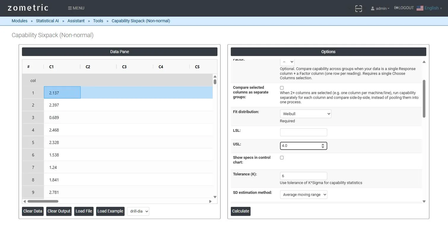
Figure 1 — Data pane with 50 surface-roughness readings in C1, Fit distribution set to Weibull, USL = 4.0.
Output Descriptions
- I Chart — individual readings in time order with UCL/CL/LCL and any Nelson-rule violations flagged.
- MR Chart — moving ranges between consecutive readings with their own UCL/CL/LCL.
- Histogram — sample histogram with the fitted nonnormal distribution's density curve and spec-limit reference lines.
- Probability Plot — sorted sample plotted on the fitted distribution's probability paper, with a reference line for visual goodness-of-fit assessment.
- Last 25 Observations panel — the most recent individual readings, for quick visual context.
- An embedded capability summary (Distribution, Shape, Scale, Pp, PPL, PPU, Ppk) rendered inside the combined figure.
- PDF export of the combined sixpack report via Download as PDF.
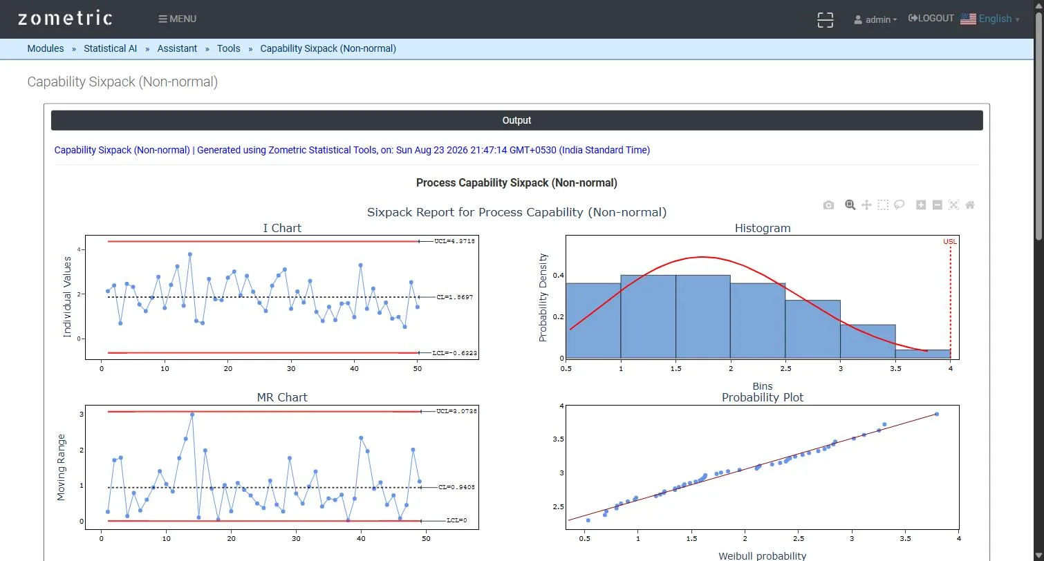
Figure 2 — The 4-panel sixpack report: I Chart, MR Chart, Histogram with fitted Weibull curve and USL line, and the Weibull probability plot.
Worked Example
A grinding operation reports surface roughness (Ra, microns) on 50 consecutive parts (column C1), right-skewed and bounded at zero — a classic Weibull-shaped process. With Fit distribution = Weibull and USL = 4.0, the sixpack shows a stable I/MR run chart (no special causes), a histogram where the fitted Weibull curve visibly tracks the right-skew the sample histogram shows, and a probability plot where the points fall close to the reference line — confirming the Weibull model is an appropriate fit before trusting the resulting capability indices.
Frequently asked questions
What is a nonnormal capability sixpack?
It is a multi-panel process-health report for data that do not follow a normal distribution, such as bounded or skewed measurements like surface roughness, particle size or time-to-failure. It combines an I chart and MR chart, a histogram with the fitted distribution, a probability plot and a capability summary, instead of forcing a normal model onto the data.
How is Ppk calculated for nonnormal data in the sixpack?
The fitted distribution's cumulative probability at the LSL and USL is converted to equivalent standard-normal z-scores, from which Pp, PPL, PPU and Ppk are reported on the familiar Cpk scale. This is the same z-score method used by the Automated Process Capability tool.
How do you check that the chosen distribution fits?
Look at the histogram, where the fitted density curve should follow the shape of the sample, and the probability plot, where a well-fitting distribution shows points close to the straight reference line. In the example, Weibull tracked the right skew of surface roughness and the points lay near the line, supporting the capability indices.
How do you run a nonnormal capability sixpack in Zometric Statistical Software?
Select the response column or columns, optionally a Factor, and choose the distribution in Fit distribution (Weibull by default). Enter the LSL, USL or both, set the tolerance K (default 6) and the moving range options, and choose which of the eight Nelson rules to check. The combined report can be downloaded as a PDF.