
Generalized Variance |S| Chart
The Generalized Variance |S| chart tracks the joint dispersion of two or more correlated variables, complementing Hotelling T-squared and MEWMA charts, which watch the mean. It needs a subgroup column with equal subgroup size n greater than the number of variables. It plots |S| per subgroup with fixed 3-sigma-equivalent limits and flags subgroups above the UCL under Rule 1.
Last reviewed
Key takeaway
A Generalized Variance |S| chart monitors the joint dispersion of two or more correlated variables by plotting the determinant of each subgroup's covariance matrix, catching variability changes mean-based charts miss.
On this page
Purpose
A Generalized Variance chart monitors the DISPERSION of two or more correlated variables jointly, complementing the Hotelling T² and MEWMA charts, which monitor whether the joint MEAN has shifted. A process can stay perfectly centered on target while becoming more erratic — its variance/covariance structure inflating — without a T² or MEWMA chart ever signaling. The Generalized Variance chart tracks the determinant of the subgroup sample covariance matrix, |S|, specifically to catch that case.
Key Capabilities
- Tracks the joint dispersion (determinant of the covariance matrix) of 2 or more correlated variables across subgroups, catching an increase or decrease in multivariate variability that a mean-based chart cannot detect.
- Requires a Subgroup indicator column, with every subgroup needing the same replicate count n, and n must exceed the number of selected variables (so the subgroup covariance matrix is estimable).
- Rule 1 (one point above the UCL) special-cause detection with a configurable K constant.
Statistical Methods
For each subgroup i (with n replicate rows and p selected variables, n > p, and every subgroup sharing the same n), the tool computes the subgroup's own sample covariance matrix and plots its determinant |S_i| — the “generalized variance” — as a single scalar summary of that subgroup's overall multivariate dispersion. A larger |S_i| means the p variables varied more (individually and/or in how their correlations shifted) within that particular subgroup.
A pooled covariance matrix S̄ (the average of all m within-subgroup covariance matrices, or those from a specified baseline set of subgroups) gives Σ̂ = det(S̄), the estimated in-control generalized variance. Two bias/variance correction constants are computed from n and p: b1 = [1/(n−1)^p] · Π_{i=1..p}(n−i), and b2 = [1/(n−1)^(2p)] · Π_{i=1..p}(n−i) · [Π_{j=1..p}(n−j+2) − Π_{j=1..p}(n−j)] — the standard moment-based constants for the sampling distribution of |S| (Montgomery, Introduction to Statistical Quality Control).
The chart uses fixed 3-sigma-equivalent limits (there is no alpha input for this chart): CL = b1·Σ̂, UCL = Σ̂·(b1 + 3√b2), LCL = max(0, Σ̂·(b1 − 3√b2)).
Only Rule 1 is evaluated — a subgroup whose |S_i| exceeds the UCL is flagged, signaling joint variability unusually large relative to the rest of the process; the default K for Rule 1 is 3.
Input Fields & Options
Field | Description |
Variables | Required. Select 2 or more correlated variables measured on each observation. |
Subgroup indicator | Required. The column identifying which subgroup each row belongs to — every subgroup must have the same number of replicate rows (n), and n must be greater than the number of selected variables. |
Check Rule 1 / K for Rule 1 | 1 point above UCL; default checked with K = 3. |
X scale | Optional custom labeling for the subgroup axis. |
Include or Exclude / Specify which rows / Row numbers | Controls which subgroups are plotted. |
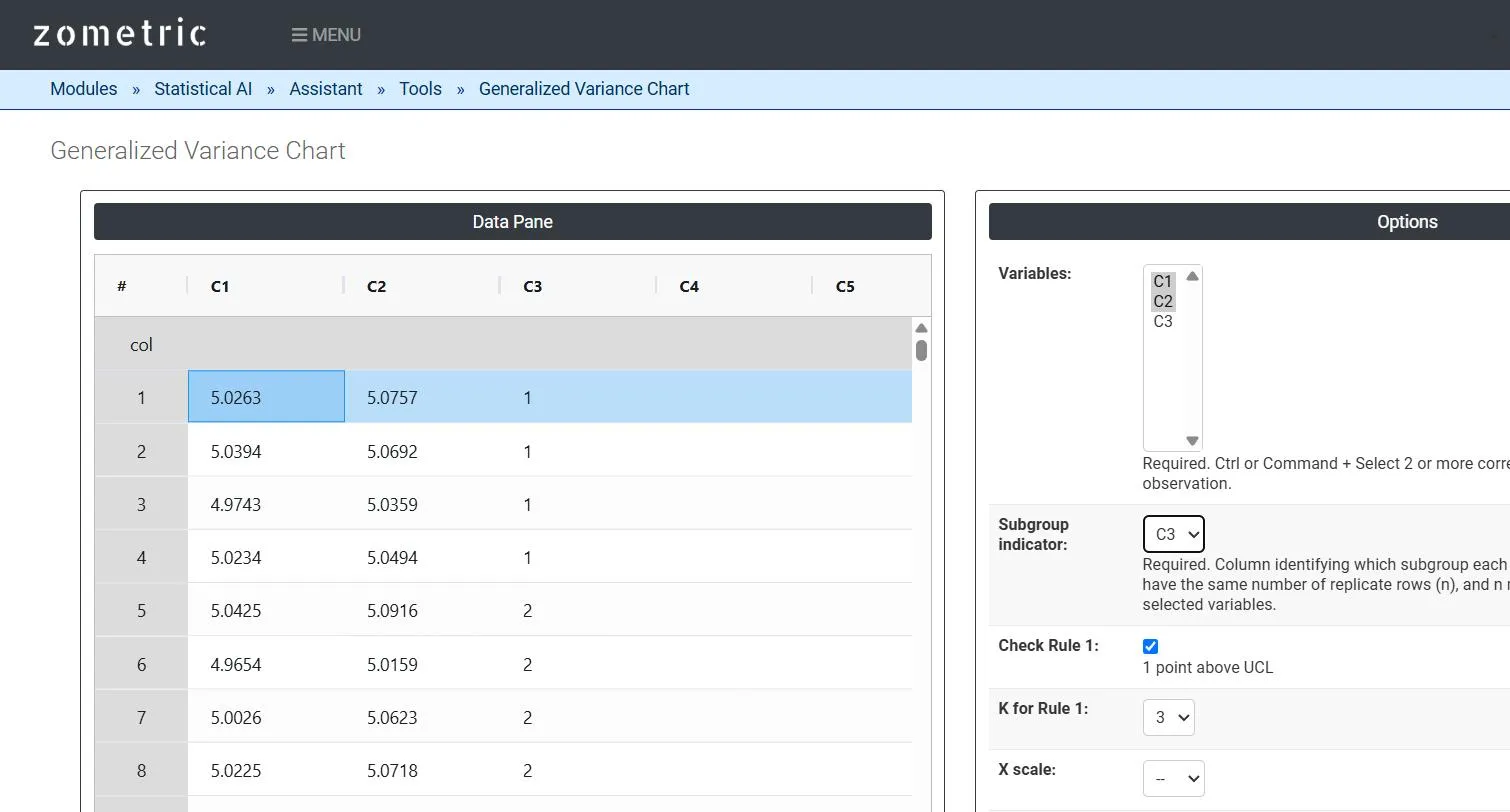
Figure 1 — 60 rows of paired pin/bore-diameter readings (C1–C2) across 15 subgroups of 4 (C3), with Variables = C1, C2 and Subgroup indicator = C3.
Output Descriptions
- Generalized Variance |S| Chart plot — the determinant of each subgroup's sample covariance matrix, plotted in subgroup order with UCL, center line and LCL.
- Any subgroup whose |S| exceeds the UCL under Rule 1 is highlighted directly on the chart.
- PDF export via Download as PDF.
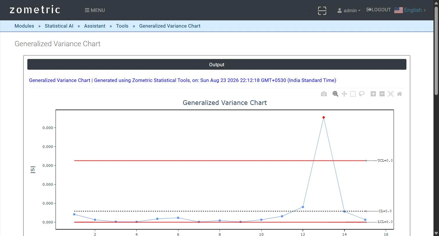
Figure 2 — Generalized Variance |S| Chart output: |S| per subgroup with UCL/CL/LCL, with the inflated-variability subgroup flagged in red.
Worked Example
A press-fit assembly depends on the joint variability of pin diameter (C1, mm) and bore diameter (C2, mm), measured on 4 parts per subgroup across 15 subgroups (C3). The first 11 subgroups are drawn from a tight, stable covariance structure while the last 4 subgroups have their variance/covariance deliberately inflated in the demo dataset (the individual means stay on target throughout). The resulting chart stays flat and in-control through subgroup 11, then subgroup 13 spikes sharply above the UCL and is flagged red under Rule 1 — catching the dispersion increase that neither a T² nor a MEWMA chart, which only watch the mean, would have detected.
Frequently asked questions
What does a generalized variance chart monitor?
It monitors the dispersion of two or more correlated variables jointly by plotting |S|, the determinant of each subgroup's sample covariance matrix. A larger |S| means the variables varied more, individually or in how their correlations shifted, within that subgroup. It catches a process that stays centred on target but becomes more erratic.
How is a generalized variance chart different from a Hotelling T-squared chart?
Hotelling T-squared and MEWMA charts monitor whether the joint mean has shifted. A process can stay centred while its variance and covariance structure inflates, without a T-squared or MEWMA chart signalling. The generalized variance chart complements them by tracking joint dispersion instead of the mean.
What subgroup size do you need for a generalized variance chart?
Every subgroup must have the same number of replicate rows, n, and n must be greater than the number of selected variables so the subgroup covariance matrix can be estimated. In the example, pin and bore diameters were measured on 4 parts per subgroup across 15 subgroups.
How are the generalized variance chart limits set?
A pooled covariance matrix from all subgroups, or a baseline set, gives the estimated in-control generalized variance. Two correction constants, b1 and b2, are computed from n and p. The chart uses fixed 3-sigma-equivalent limits with no alpha input, and only Rule 1, one point above the UCL with a default K of 3, is evaluated.