
Multiple Variables Process Capability
Multiple Variables Process Capability scores two or more columns, such as cavities, machines or lines, against one shared LSL/USL and optional Target. Use it to find the worst-performing process without comparing separate reports. Every variable is assumed Normal, with no per-variable normality test. Output is one comparison table with N, Mean, StDev, Pp, Ppk, Cpm and PPM, plus a histogram per variable.
Last reviewed
Key takeaway
Multiple Variables Process Capability compares several parallel processes, such as mold cavities, machines or lines, against one shared specification in a single Pp, Ppk and Cpm table to show which one is worst.
On this page
Purpose
Multiple Variables Process Capability answers a specific, common question that the app's existing capability tools could only answer indirectly: when the same characteristic is measured across several parallel variables — different cavities of an injection mold, different machines, different lines — against one shared specification, which one is worst? Rather than running N separate capability reports and comparing them by eye, this tool produces ONE unified side-by-side comparison table and one set of histograms, so every variable's Cp/Cpk-family indices sit in the same table.
Key Capabilities
- Select any 2 or more columns and get one aggregated comparison table instead of N stacked reports.
- A single LSL/USL pair is applied uniformly to every selected variable, so the comparison is always apples-to-apples against the same specification.
- Optional shared Target adds the Cpm index per variable to the same comparison table.
- Per-variable histograms with the shared spec limits overlaid, alongside the aggregated table.
- Configurable K-sigma tolerance multiplier, consistent with the app's other capability tools.
Statistical Methods
Each selected variable/column is treated as an independent process, run through the same Normal-capability engine used by the Automated Process Capability tool's Normal path. For each one, σ_overall is estimated via the moving-range method (MRbar/d2, or median-moving-range), and the standard z-based Performance index family is computed: Pp = (USL − LSL) / (K·σ), Ppu = (USL − x̄) / ((K/2)·σ), Ppl = (x̄ − LSL) / ((K/2)·σ), Ppk = min(Ppu, Ppl), with the default K = 6. Every variable always assumes Normality here — there is no per-variable normality test or nonnormal routing in this tool.
When a shared Target is supplied, Cpm is additionally computed per variable: Cpm = (USL − LSL) / (K·√(mean((x − Target)²))), penalizing a variable whose mean sits off-target even if its spread alone would otherwise look capable.
Because every variable is scored against the identical LSL/USL (and Target, when supplied), the resulting Ppk and Cpm values are directly comparable across variables — the variable with the lowest Ppk (or Cpm) in the comparison table is the worst-performing one relative to the shared spec.
PPM Expected is computed from the fitted Normal distribution's tail probability beyond each spec limit for that variable; PPM Observed is the empirical fraction of that variable's own sample falling outside the spec limits — letting a user spot cases where the two disagree (a sign the Normal-distribution assumption may not hold for that particular variable).
Input Fields & Options
Field | Description |
Process variables | Required. Select 2 or more columns to compare — each column is treated as its own process. |
LSL / USL | Applied to every selected variable. |
Target | Optional. Adds the Cpm index per variable to the comparison table. |
Tolerance (K) | Multiplier applied to sigma when forming the capability tolerance band; default 6. |
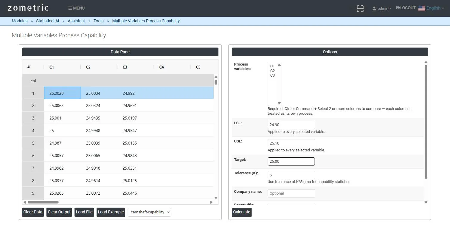
Figure 1 — Data pane with bore-diameter readings from 3 cavities in C1–C3, all three selected as Process variables, with a shared LSL/USL/Target.
Output Descriptions
- Comparison table — one row per selected variable with N, Mean, StDev, Pp, Ppl, Ppu, Ppk, Cpm (when Target is supplied), PPM Expected and PPM Observed, all against the same shared spec limits.
- Per-variable histogram — each variable's own distribution with the shared LSL/Target/USL reference lines and a fitted Normal curve.
- PDF export of the full comparison report via Download as PDF.
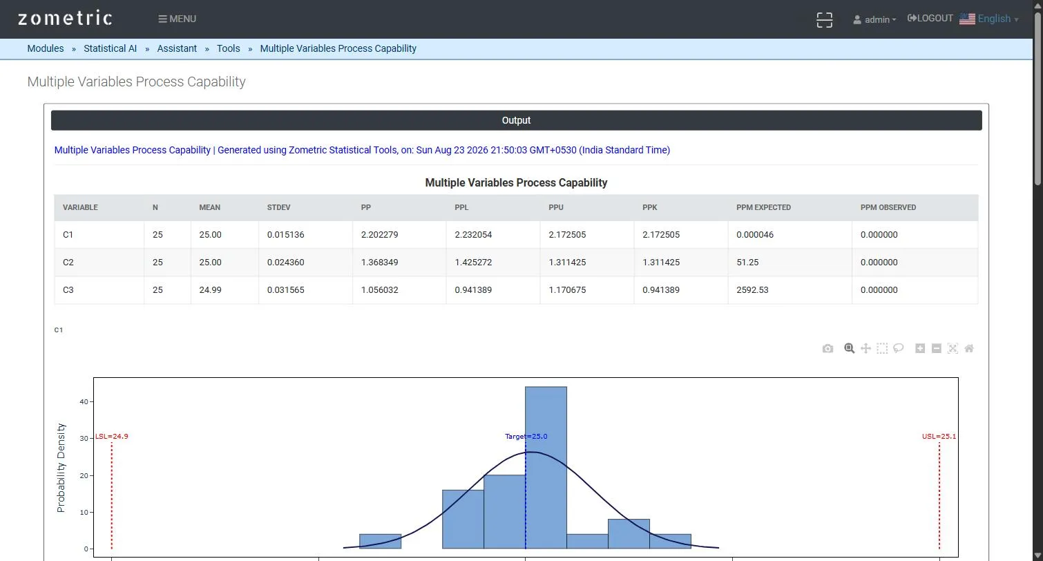
Figure 2 — The unified comparison table (N, Mean, StDev, Pp, Ppl, Ppu, Ppk, Cpm, PPM Expected, PPM Observed per variable) with the first variable's histogram.
Worked Example
An injection-molding tool has 3 cavities producing the same part; bore diameter (mm) is measured on 25 parts from each cavity (C1 = Cavity 1, C2 = Cavity 2, C3 = Cavity 3), against a shared LSL = 24.90, USL = 25.10, Target = 25.00. The comparison table shows Cavity 1 with the tightest spread (Ppk ≈ 2.17, Cpm ≈ 2.24) and Cavity 3 visibly worse (Ppk ≈ 0.94) — immediately flagging Cavity 3 as the one needing attention, without having to run and manually compare three separate reports.
Frequently asked questions
What is Multiple Variables Process Capability?
It is a capability analysis that compares the same characteristic measured across several parallel variables, such as different mold cavities, machines or lines, against one shared specification. Instead of separate reports, it produces one side-by-side comparison table of Pp, Ppl, Ppu, Ppk, Cpm and PPM values, so the worst-performing variable is easy to identify.
How do you identify the worst process in a multiple variables capability study?
Because every variable is scored against the identical LSL, USL and Target, the Ppk and Cpm values are directly comparable. The variable with the lowest Ppk, or the lowest Cpm when a Target is supplied, is the worst-performing one relative to the shared specification and should be investigated first.
Does Multiple Variables Process Capability assume normality?
Yes. Every variable is analysed with a Normal-capability calculation and there is no per-variable normality test or nonnormal routing. Comparing PPM Expected, from the fitted Normal tail, with PPM Observed, the actual fraction outside spec, helps spot variables where the two disagree, a sign that the Normal assumption may not hold.
What does Cpm add to the comparison?
When a shared Target is supplied, Cpm is computed for each variable as (USL - LSL) divided by K times the root mean squared deviation from Target. It penalises a variable whose mean sits off-target, even if its spread alone would otherwise look capable.