
Multiple Variables Process Capability (Nonnormal)
This tool compares capability of two or more columns against one specification when data are skewed, such as particle size, flatness or impurity. It fits one chosen model from fifteen, including Weibull, Lognormal, Box-Cox and Johnson, to each column, using the Z-Score or ISO method. Each column needs at least 4 values. Output is a table of Pp, PPL, PPU, Ppk and PPM, plus histograms.
Last reviewed
Key takeaway
Multiple Variables Process Capability (Nonnormal) compares several processes against one specification when data are not normal, fitting the same distribution to each and listing Pp, Ppk and PPM side by side.
On this page
Purpose
Multiple Variables Process Capability (Nonnormal) compares the capability of several processes, lines, machines or cavities against one specification when the data are not normally distributed. It fits the same distribution to each column separately and puts Pp, PPL, PPU, Ppk and the expected and observed parts per million out of specification side by side in one table, with a histogram for each column. Use it for skewed characteristics such as particle size, flatness, runout or impurity, where a normal-based Ppk misjudges the tail, and you want to rank the processes.
Key Capabilities
- Two or more columns, each treated as its own process and fitted independently.
- Fifteen models: Weibull, Exponential, Logistic, Loglogistic, Largest and Smallest Extreme Value, 2-Parameter Exponential, 3-Parameter Weibull, Gamma, Lognormal, 3-Parameter Lognormal, 3-Parameter LogLogistic, Box-Cox and Johnson transformations, and a Mixed Distribution (ISO 22514-2).
- Z-Score or ISO percentile method for the indices.
- One-sided or two-sided specifications applied to every column.
- Comparison table with Pp, PPL, PPU, Ppk, PPM Expected and PPM Observed, and a histogram of each column with the specification limits and fitted curve.
Statistical Methods
For each column the chosen distribution is fitted by maximum likelihood (Weibull, Gamma and Exponential with the threshold fixed at 0; the 3-parameter models estimate it). Lognormal uses the mean and standard deviation of the log data. Box-Cox and Johnson transform the data to normal and work on the transformed scale; the Mixed Distribution fits a mixture of normal distributions, with the number of components chosen by BIC unless fixed. Each column needs at least 4 values.
Z-Score method (default): the fitted probabilities beyond each limit are turned into normal scores, Z_USL = Φ⁻¹(F(USL)) and Z_LSL = Φ⁻¹(F(LSL)), where F is the fitted cumulative distribution. Then PPU = Z_USL / 3, PPL = −Z_LSL / 3, Pp = (Z_USL − Z_LSL) / 6 and Ppk = min(PPL, PPU). ISO method: the indices use the fitted percentiles X₀.₁₃₅, X₅₀ and X₉₉.₈₆₅ (the points that cover the same ±3σ share as a normal): Pp = (USL − LSL) / (X₉₉.₈₆₅ − X₀.₁₃₅), PPL = (X₅₀ − LSL) / (X₅₀ − X₀.₁₃₅), PPU = (USL − X₅₀) / (X₉₉.₈₆₅ − X₅₀). With one limit only, Pp is not given and Ppk is the one-sided index.
PPM Expected is the fitted share of the population beyond the limits, times 1,000,000; PPM Observed is the share of the sample values beyond them. These are overall (long-term) indices from all the data. They are only as good as the distribution: the same model is applied to every column, so check the fit of each one (for example with Individual Distribution Identification) before comparing the columns.
Input Fields & Options
Field | Description |
Process variables | Required. Two or more numeric columns to compare; each is fitted on its own. |
Fit distribution | Required. One of the fifteen models listed above (default Weibull), applied to every column. |
Mixture components | Only for Mixed Distribution (ISO 22514-2): Auto (BIC-selected, default) or 2 to 6 components. |
Method of analysis | Z-Score (default) or ISO. |
LSL / USL | Specification limits applied to every column; at least one is required, and LSL must be below USL. |
Company name / Report title | Optional text for the report; default title Multiple Variables Process Capability (Nonnormal). |
Data Options: Subset (optional) | Exclude matching rows (default) or Include only matching rows, by row numbers (e.g. 3,7,12-15) and/or a condition. |
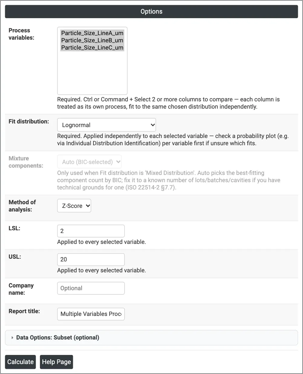
Figure 1 — Options for the example: particle size of three lines, Lognormal, Z-Score method, LSL 2 µm and USL 20 µm.
Output Descriptions
- Multiple Variables Process Capability (Nonnormal) — one row per column: Variable, N, Distribution, Pp, PPL, PPU, Ppk, PPM Expected and PPM Observed.
- Histogram of <distribution> Distribution — one per column, under the column name, with the LSL and USL and the fitted density curve.
- PDF export via Download.
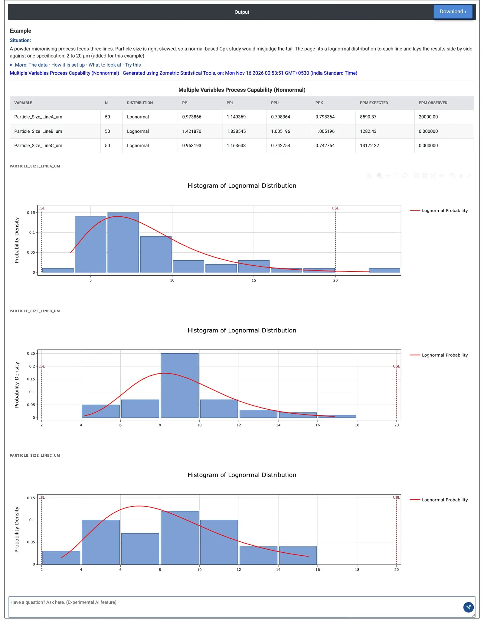
Figure 2 — Comparison table and lognormal histograms for the three lines: Ppk 0.798 for line A, 1.005 for line B and 0.743 for line C, with PPU below PPL on every line; only line A has a sample above the USL.
Worked Example
A powder micronising process feeds three lines, and particle size is right-skewed (median about 7 to 9 µm, with a long tail to coarse particles). The process engineer wants to compare the lines against a specification of 2 to 20 µm using 50 samples from each. Process variables = Particle_Size_LineA_um, Particle_Size_LineB_um and Particle_Size_LineC_um, Fit distribution = Lognormal, Method of analysis = Z-Score, LSL = 2, USL = 20.
Line A has Ppk 0.798 and 8,590 PPM expected out of specification; one sample (22.11 µm) is already above 20 µm, so 20,000 PPM are observed. Line B is the best, with Ppk 1.005 and 1,282 PPM expected, but still below the usual target of 1.33. Line C is the riskiest, with Ppk 0.743 and 13,172 PPM expected. On every line PPU is lower than PPL: the risk is coarse particles above 20 µm, not fines below 2 µm, so improvement work should target the coarse tail, starting with line C. The histograms show the same picture: each fitted curve has its long tail towards the USL, and on line A one bar lies beyond it.
The model matters. With the ISO method the Ppk values fall to 0.694, 1.008 and 0.619, with the same ranking. With a Weibull fit, PPL becomes the lower index on every line and the ranking changes (Ppk 0.641, 0.948 and 0.798, line A now worst). Anderson-Darling statistics computed separately from this page favour the lognormal for lines A and B (0.79 against 2.17, and 0.63 against 1.34) but the Weibull for line C (0.20 against 0.55), so the lines should be checked one by one before the ranking is used for decisions.
Frequently asked questions
When should you use nonnormal capability analysis for multiple variables?
Use it to compare and rank the capability of several processes, lines, machines or cavities against one specification when the data are not normally distributed. Typical examples are skewed characteristics such as particle size, flatness, runout or impurity, where a normal-based Ppk misjudges the tail of the distribution.
What is the difference between the Z-Score and ISO methods?
The Z-Score method converts the fitted probabilities beyond each limit into normal scores and divides by 3 to give PPU and PPL. The ISO method uses the fitted 0.135th, 50th and 99.865th percentiles in place of the normal plus or minus 3 sigma spread. Both can give different Ppk values, as the worked example shows, though the ranking may stay the same.
Why does the choice of distribution matter in nonnormal capability?
The indices are only as good as the fitted distribution, and the same model is applied to every column. In the worked example, switching from Lognormal to Weibull changed which index was lower and changed the ranking of the lines. Check the fit of each column, for example with Individual Distribution Identification, before comparing them.
What is the difference between PPM Expected and PPM Observed?
PPM Expected is the fitted distribution's share of the population beyond the specification limits, times 1,000,000. PPM Observed is the share of the actual sample values beyond the limits. Both are overall, long-term measures calculated from all the data in each column.