
Poisson Regression
Poisson regression models counts of events in a fixed amount of time, area or product against continuous and categorical predictors. Use it instead of ordinary regression because counts cannot be negative and their spread grows with the mean. The response is assumed to follow a Poisson distribution, with a log, square root or identity link. Outputs include coefficients, analysis of deviance, goodness-of-fit tests and residual plots.
Last reviewed
Key takeaway
Poisson regression is a generalised linear model that relates a count response, such as defects per shift or breakdowns per month, to continuous and categorical predictors, fitted by maximum likelihood.
On this page
Purpose
Poisson Regression relates a count response, such as defects per shift, breakdowns per month or flaws per panel, to continuous and categorical predictors. Use it instead of ordinary regression when the response is a count of events in a fixed amount of time, area or product: the counts cannot be negative and their spread grows with their mean, which least squares does not allow for.
Key Capabilities
- Continuous and categorical predictors, with interactions and squared terms from the term list.
- Log (default), square root or identity link.
- Stepwise, forward selection or backward elimination of terms, with terms forced into every model.
- Coefficients with confidence intervals and VIF, regression equations for each level of a categorical predictor, model summary and goodness-of-fit tests.
- Analysis of deviance by Wald or likelihood-ratio tests (adjusted or sequential).
- Unusual observations, residual plots, main effects and interaction plots, contour and surface plots of fitted counts.
- Prediction at settings you enter and a response optimizer.
Statistical Methods
The response is assumed to follow a Poisson distribution with mean μ that depends on the predictors through the link: with the log link, ln μ = b₀ + b₁x₁ + … , so each coefficient multiplies the expected count by exp(b) per unit of its predictor. The model is a generalised linear model fitted by maximum likelihood (iteratively reweighted least squares). Categorical predictors use (1, 0) coding against a reference level, by default the first level in sort order. Rows with a missing value are dropped; a frequency column repeats rows and a weights column gives variance weights.
The coefficient table gives Wald z-values (Coef / SE Coef) and confidence intervals. The analysis of deviance tests each term: by default with a Wald chi-square (z² for a continuous term, a joint test for the dummy columns of a categorical term); with the LR test, by the change in deviance when the term is dropped from the full model (adjusted, Type III) or added in order (sequential, Type I). Deviance R-Sq = 1 − residual deviance / null deviance.
Goodness-of-fit tests compare the deviance and the Pearson chi-square with a chi-square distribution on the error degrees of freedom. A small p-value, or a Mean (deviance / DF) well above 1, means the counts vary more than a Poisson model allows (overdispersion), and the p-values for the terms are then too small. Observations with a standardised residual beyond ±2 are flagged R, and those with leverage above 3p/n are flagged X.
Input Fields & Options
Field | Description |
Response | Column of counts. Required. |
Continuous Predictors / Categorical Predictor | Numeric and text (or coded) predictor columns; at least one. Ctrl or Command + click to select several. |
Model terms (optional) | Term list: tick terms, or use Add all, Interactions and Powers up to the order chosen in Terms through order (2 or 3). Untick In model to remove a linear term while keeping its interactions. |
Reference level (optional) | For categorical predictors, “Predictor Level”, comma-separated. Default: first level in sort order. |
Stepwise method | None (default), Stepwise, Forward selection or Backward elimination; with Alpha to enter and Alpha to remove (0.15), hierarchy rules, Terms in every model (E), Initial model terms (I) and Model selection details. |
Frequency (optional) / Weights (optional) | Columns of row frequencies and of weights. |
Link function | Log (default), Square root or Identity. |
Confidence level / Type of confidence interval | Default 95, Two-sided; or Lower bound or Upper bound. |
Fits and diagnostics for all observations | Lists fit and residual for every row, not only unusual ones. |
Test for ANOVA table / Type of deviance (LR test only) | Wald test (default) or LR test; for LR, Adjusted (Type III, default) or Sequential (Type I). |
Residuals for diagnostics/plots | Deviance (default) or Pearson. |
Histogram of residuals / Normal probability plot of residuals / Residuals versus fits / Residuals versus order / Four in one / Residuals versus the variables | Residual plots. |
Main effects plot / Interaction plot | Fitted count against each predictor, the others held at their mean or reference level. |
Contour plot / Surface plot / Overlaid contour plot of fitted values | Need X1 and X2 axis variables; the overlaid contour plot also needs Response low and Response high. |
Prediction / Response Optimizer | Add a panel to predict the mean count (with SE and confidence interval) at settings you enter, or to search for settings that meet a count goal. |
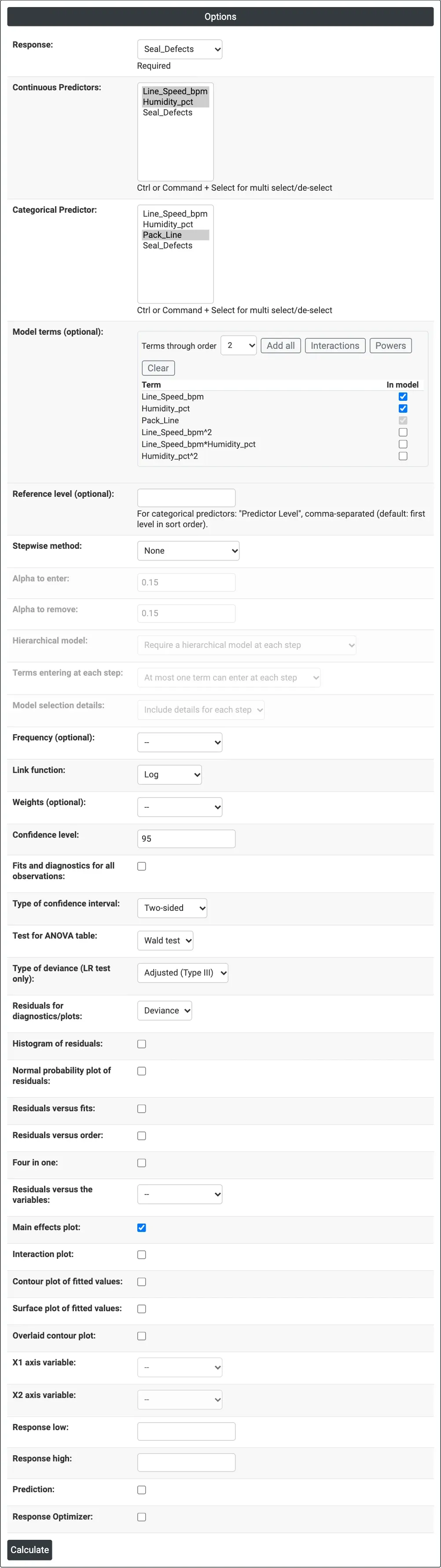
Figure 1 — Options for the bag seal example: Seal_Defects as the response, line speed and humidity as continuous predictors, packing line as a categorical predictor, main effects plot ticked.
Output Descriptions
- Method — link function, categorical coding and rows used.
- Response Information — N, mean, standard deviation, minimum and maximum of the counts.
- Coefficients — Coef, SE Coef, Z-Value, P-Value, confidence limits and VIF.
- Regression Equation — the linear predictor Y' (ln of the expected count with the log link) for each level of the categorical predictors.
- Model Summary — deviance R-Sq, Adj R-Sq, AIC, AICc and BIC.
- Goodness-of-Fit Tests — deviance and Pearson chi-square tests.
- Fits and Diagnostics for Unusual Observations.
- Analysis of Deviance — chi-square and p-value for the regression and each term.
- Stepwise selection table, residual, factorial, contour and surface plots, prediction and optimizer panels when selected.
- PDF export via Download.
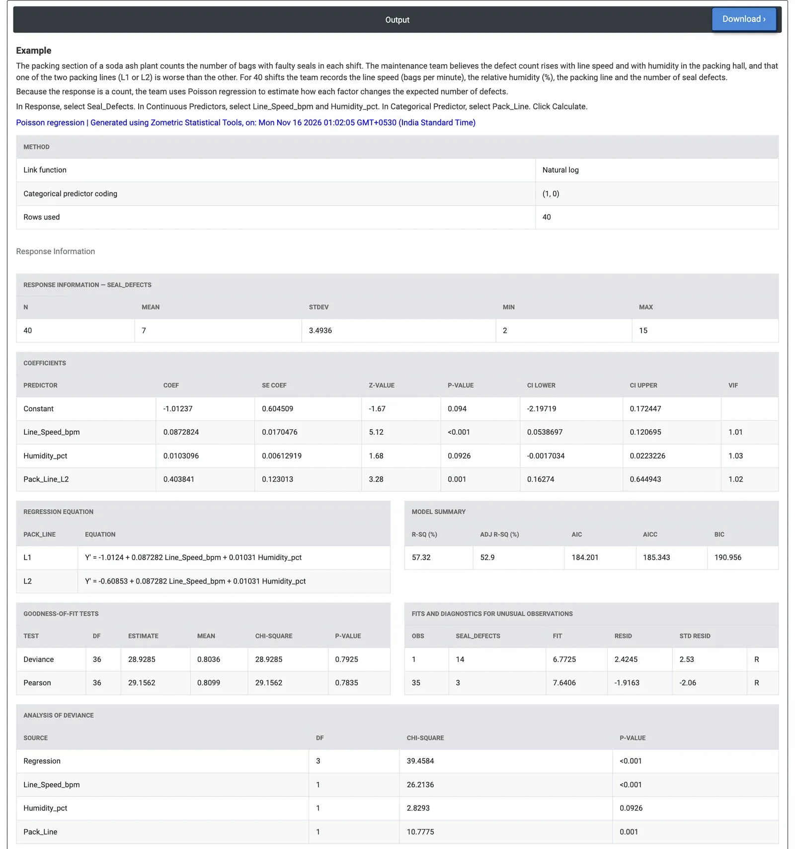
Figure 2 — Poisson regression of seal defects per shift: line speed (p < 0.001) and packing line (p = 0.001) matter, humidity does not at the 5% level (p = 0.0926).
Worked Example
The packing section of a soda ash plant counts the bags with faulty seals in each shift. For 40 shifts the team records the line speed (bags per minute), the humidity in the packing hall (%), the packing line (L1 or L2) and the number of seal defects (2 to 15, mean 7). They select Seal_Defects as the response, line speed and humidity as continuous predictors and Pack_Line as the categorical predictor, and keep the log link.
Line speed has the strongest effect (Wald chi-square 26.21, p < 0.001): its coefficient 0.0873 means each extra bag per minute multiplies the expected defects by exp(0.0873) = 1.09, and 5 bags per minute faster by about 1.55. Line L2 has coefficient 0.404 (p = 0.001), so at the same speed and humidity it makes about 1.50 times as many seal defects as L1. Humidity points the same way (about 11% more defects per 10% RH) but is not significant at the 5% level (p = 0.0926).
The model fits the counts: deviance chi-square 28.93 on 36 DF (p = 0.7925) and Pearson 29.16 (p = 0.7835), with Mean below 1, so there is no sign of overdispersion. Two shifts are flagged: shift 1 with 14 defects against a fit of 6.8, and shift 35 with 3 against 7.6. The team looks first at the seal jaws on L2 and at the speed set point, and keeps collecting humidity data before deciding on dehumidification.
Frequently asked questions
When should you use Poisson regression instead of ordinary least squares regression?
Use Poisson regression when the response is a count of events in a fixed amount of time, area or product, such as defects per shift or breakdowns per month. Counts cannot be negative and their spread grows with their mean, which least squares regression does not allow for. Poisson regression handles this as a generalised linear model fitted by maximum likelihood.
How do you interpret Poisson regression coefficients?
With the default log link, ln of the expected count equals b0 + b1x1 + ..., so each coefficient multiplies the expected count by exp(b) per unit increase in its predictor. For example, a line speed coefficient of 0.0873 means each extra bag per minute multiplies expected defects by exp(0.0873) = 1.09. Categorical predictors are compared against a reference level.
How do you check for overdispersion in Poisson regression?
The goodness-of-fit tests compare the deviance and the Pearson chi-square with a chi-square distribution on the error degrees of freedom. A small p-value, or a Mean (deviance divided by DF) well above 1, means the counts vary more than a Poisson model allows. In that case the p-values for the model terms are too small and should not be trusted.
How are unusual observations flagged in Poisson regression?
Observations with a standardised residual beyond plus or minus 2 are flagged R, and observations with leverage above 3p/n are flagged X. They are listed in the Fits and Diagnostics for Unusual Observations table, and residual plots such as residuals versus fits and a normal probability plot of residuals can be added to examine them further.