
Probability Distribution Plot
The Probability Distribution Plot draws a theoretical distribution's density, mass or cumulative curve from entered parameters, without data. It covers twelve distributions, including Normal, t, Chi-Square, F, Weibull, Lognormal, Binomial and Poisson. Use it to see a distribution's shape, explain a sampling plan or test statistic, or read off probabilities. Continuous distributions appear as curves; Binomial and Poisson appear as bars.
Last reviewed
Key takeaway
A probability distribution plot draws the probability density (or mass) or cumulative distribution curve of a theoretical distribution, such as Normal, Weibull or Binomial, from parameters you enter, with no data needed.
On this page
Purpose
The Probability Distribution Plot draws the curve of a theoretical distribution for parameters you enter: its probability density (or, for counts, its probability mass) or its cumulative distribution. No data are needed. Use it to see what a distribution looks like before using it, to explain a sampling plan or a test statistic, or to read off how likely a count or a measurement is under an assumed model, for example the number of defectives in a sample of 50 when the process runs at 4% defective.
Key Capabilities
- Twelve distributions: Normal, Student's t, Chi-Square, F, Exponential, Weibull, Lognormal, Uniform, Gamma, Beta, Binomial and Poisson.
- Probability density/mass function or cumulative distribution function.
- Continuous distributions drawn as a smooth curve (the density is shaded); Binomial and Poisson drawn as bars at each whole number.
- The horizontal range is chosen automatically to cover the distribution from its 0.05th to its 99.95th percentile.
- Title generated from the distribution and curve, or your own title.
Statistical Methods
The tool builds the chosen distribution from the parameters and evaluates it with standard formulas. The parameters are: Normal — Parameter 1 = mean, Parameter 2 = standard deviation; Student's t and Chi-Square — degrees of freedom; F — numerator and denominator degrees of freedom; Exponential — scale (the mean); Weibull and Gamma — shape and scale; Lognormal — location and shape, i.e. the mean and standard deviation of ln(X); Uniform — lower and upper bound; Beta — the two shape parameters α and β; Binomial — number of trials n and event probability p; Poisson — mean λ. Distributions with one parameter use only Parameter 1.
For a continuous distribution the curve is evaluated at 500 evenly spaced points between its 0.05th and 99.95th percentiles. For the Binomial and Poisson it is evaluated at every whole number in that range: the probability mass P(X = k) gives the height of each bar, and the cumulative function P(X ≤ k) gives the height of each bar in the CDF plot. For a density, the area under the curve over an interval is the probability of falling in that interval; the CDF gives that probability directly as a difference of two heights.
Input Fields & Options
Field | Description |
Distribution | Required. Normal, Student's t, Chi-Square, F, Exponential, Weibull, Lognormal, Uniform, Gamma, Beta, Binomial or Poisson. |
Parameter 1 | Meaning depends on the distribution: e.g. mean for Normal, degrees of freedom for t and Chi-Square, shape for Weibull and Gamma, number of trials for Binomial, mean for Poisson. |
Parameter 2 | Only used by two-parameter distributions: e.g. standard deviation for Normal, scale for Weibull and Gamma, event probability for Binomial. |
Plot | Probability density/mass function (default) or Cumulative distribution function. |
Title | Optional. Defaults to a title generated from the distribution and curve chosen. |
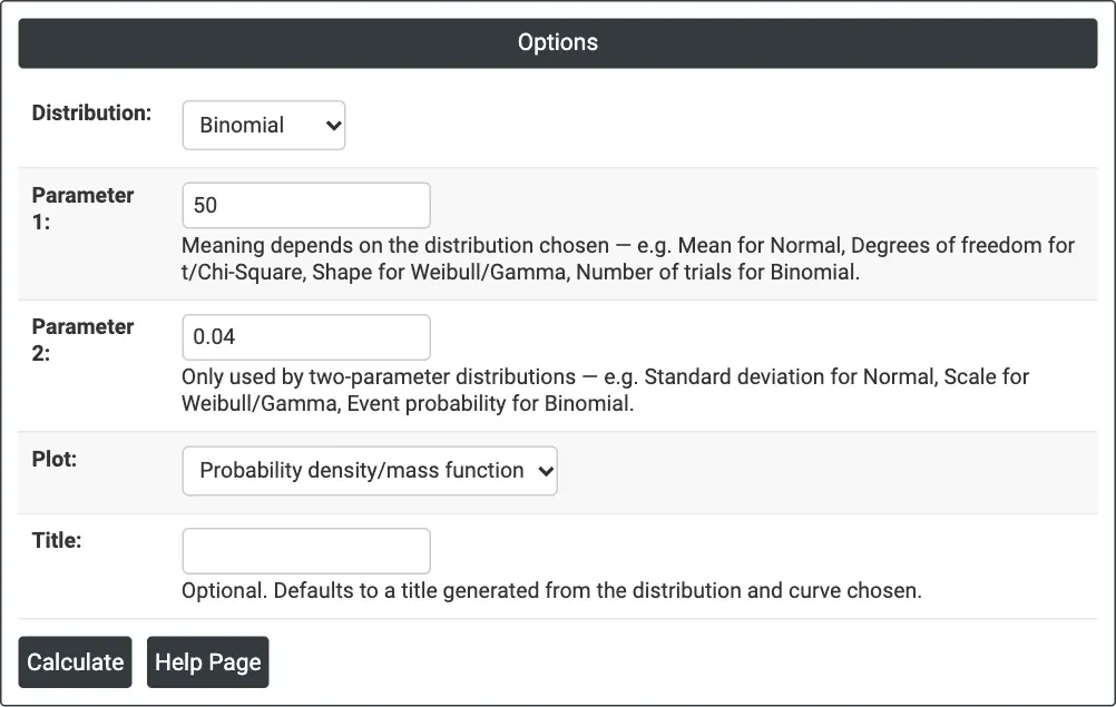
Figure 1 — Options for the example: Binomial distribution with 50 trials and event probability 0.04.
Output Descriptions
- <Distribution> Distribution — Probability Density: the density curve (axis labelled Probability density); for Binomial and Poisson, <Distribution> Distribution — Probability Mass, with the probability of each count as bars (axis labelled Probability).
- <Distribution> Distribution — Cumulative Distribution: the cumulative probability P(X ≤ x).
- PDF export via Download.
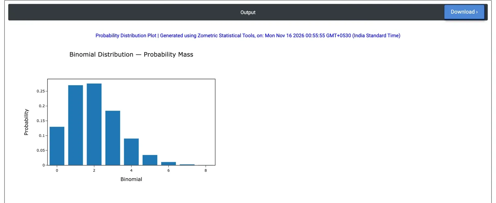
Figure 2 — Probability of 0 to 8 defectives in a sample of 50 when the process is 4% defective (Binomial, n = 50, p = 0.04).
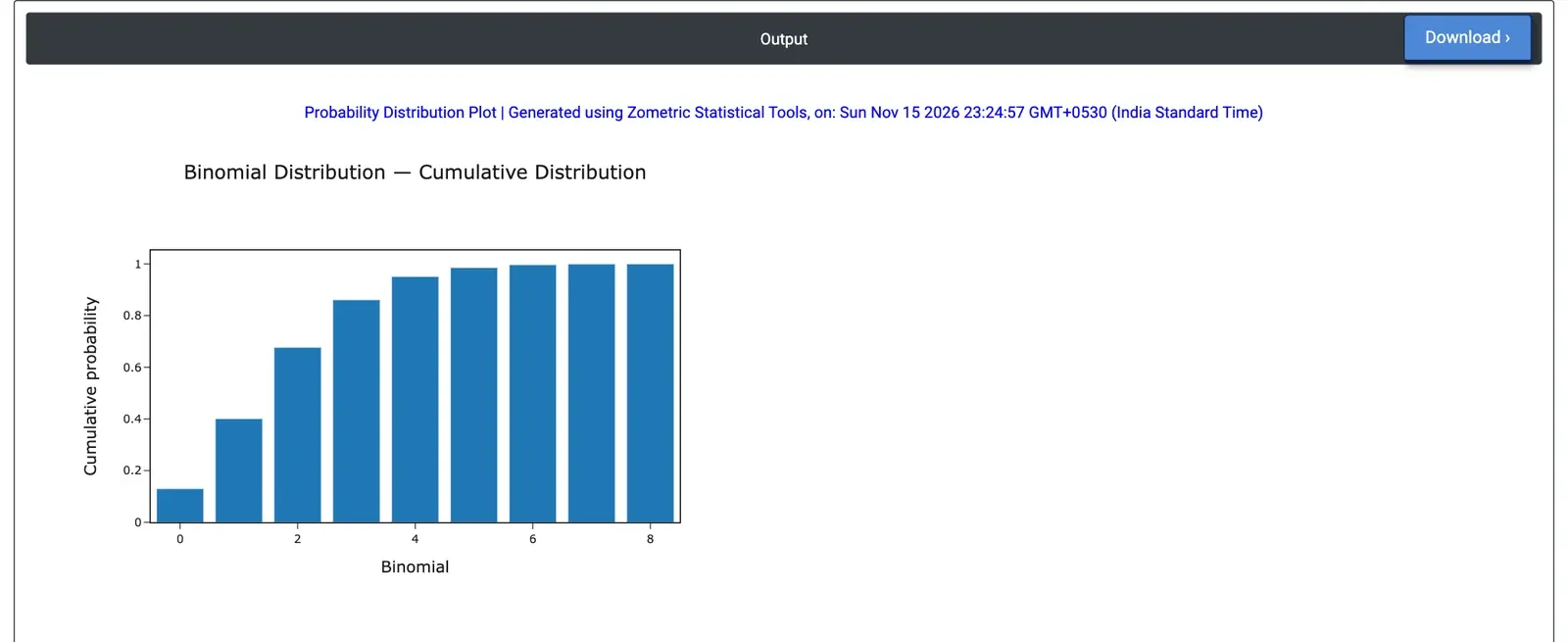
Figure 3 — The same distribution with Plot = Cumulative distribution function: P(X ≤ k) for k = 0 to 8.
Worked Example
A supplier's process runs at about 4% defective. Incoming inspection takes a sample of 50 parts from each lot, and the quality engineer wants to know how many defectives to expect and how often a lot from this process would show 3 or more. Distribution = Binomial, Parameter 1 = 50 (trials), Parameter 2 = 0.04 (event probability), Plot = Probability density/mass function.
The bars run from 0 to 8 defectives. The most likely counts are 1 (probability 0.271) and 2 (0.276), matching the mean of n·p = 2. A sample with no defectives occurs 13.0% of the time, so a clean sample says little about whether the process has improved. Switching Plot to Cumulative distribution function gives P(X ≤ 2) = 0.677, so 32.3% of samples from this process would contain 3 or more defectives, and 13.9% would contain 4 or more.
For the inspection plan this means an acceptance number of 2 would reject about one lot in three even when the supplier is running at its normal 4%. If such lots should usually pass, the acceptance number must be higher or the sample plan redesigned; Acceptance Sampling and the AQL tools work this out against the agreed quality levels.
Frequently asked questions
What is a probability distribution plot used for?
It shows what a theoretical distribution looks like for given parameters, without any data. Use it to see a distribution's shape before using it, to explain a sampling plan or a test statistic, or to read off how likely a count or measurement is under an assumed model, such as the number of defectives in a sample of 50 from a process at 4% defective.
Which distributions can a probability distribution plot show?
Twelve: Normal, Student's t, Chi-Square, F, Exponential, Weibull, Lognormal, Uniform, Gamma, Beta, Binomial and Poisson. Parameter 1 and Parameter 2 depend on the distribution, for example mean and standard deviation for the Normal, shape and scale for Weibull and Gamma, and number of trials and event probability for the Binomial. One-parameter distributions use only Parameter 1.
What is the difference between the PDF and CDF plots?
The probability density (or mass) function shows the height of the distribution at each value; for a density, the area under the curve over an interval is the probability of falling in it, and for Binomial or Poisson each bar is P(X = k). The cumulative distribution function shows P(X less than or equal to x), so a probability is a difference of two heights.
How do you read a binomial probability distribution plot?
In a worked example with 50 trials and an event probability of 0.04, the most likely counts are 1 (0.271) and 2 (0.276), matching the mean n times p = 2, and zero defectives occurs 13.0% of the time. The cumulative plot gives P(X less than or equal to 2) = 0.677, so 32.3% of samples would contain 3 or more defectives.