
Probability Plot
The Probability Plot tests whether data fit a distribution by plotting ordered values on a scale where the distribution appears as a straight line, with confidence bounds. It supports nine distributions, including Normal, Lognormal, Weibull and Exponential, and reports the Anderson-Darling statistic and p-value for each. Use it before capability analysis, control limits or t-tests that assume normality, and to choose a reliability distribution.
Last reviewed
Key takeaway
A probability plot checks whether data follow a chosen distribution, most often the normal, by plotting ordered data on a scale where that distribution is a straight line, with an Anderson-Darling statistic and p-value.
On this page
Purpose
The Probability Plot checks whether data follow a chosen distribution, most often the normal distribution. The ordered data are plotted on a scale on which the chosen distribution appears as a straight line: if the points follow the line, the distribution fits. Use it before capability analysis, control limits, tolerance intervals or t-tests that assume normality, and to choose a distribution (Weibull, lognormal, exponential) for reliability or non-normal capability work.
Key Capabilities
- Nine distributions: Normal, Lognormal, Weibull, Exponential, 2-Parameter Exponential, Smallest Extreme Value, Largest Extreme Value, Logistic and Loglogistic.
- Fitted reference line with pointwise confidence bounds at a chosen level (default 95%).
- Anderson-Darling (AD) statistic and its p-value in the legend for every distribution, so the fits can be compared.
- Several variables overlaid on one plot, or one variable split into groups by a By column, each with its own fitted line.
- Logarithmic data axis for the Lognormal, Weibull and Loglogistic, as on standard probability paper.
Statistical Methods
For each variable or group (at least 3 values), the data are sorted, x₍₁₎ ≤ … ≤ x₍ₙ₎, and each is given the plotting position pᵢ = (i − 0.3) / (n + 0.4), Benard's median-rank approximation. The vertical axis is the inverse CDF of the chosen distribution, labelled in percent, so a sample from that distribution falls close to a straight line. The reference line is the fitted CDF: for the Normal, the sample mean and the standard deviation (n − 1 divisor); for the other distributions, maximum likelihood, with the threshold fixed at 0 for the Lognormal, Weibull, Exponential and Loglogistic (these need positive values).
The confidence bounds are drawn through each point: at level C, the lower bound is the α/2 quantile of a Beta(i, n − i + 1) distribution and the upper bound the 1 − α/2 quantile of a Beta(i + 1, n − i) distribution, where α = 1 − C/100. Points that leave the bounds are evidence against the distribution.
The Anderson-Darling statistic AD = −n − (1/n) Σ (2i − 1)[ln F(x₍ᵢ₎) + ln(1 − F(x₍ₙ₊₁₋ᵢ₎))] measures how far the points are from the fitted CDF F, with extra weight in the tails; smaller is better. The legend shows this unadjusted AD for every distribution, as Minitab does. The p-value comes from a modified statistic, as in D'Agostino and Stephens: for the Normal and Lognormal (on the logs), AD·(1 + 0.75/n + 2.25/n²) converted with Stephens' approximation; for the Weibull and the two extreme value distributions, AD·(1 + 0.2/√n); for the Exponential, AD·(1 + 0.6/n); for the Logistic and Loglogistic, AD·(1 + 0.25/n). The last three are looked up in Stephens' tables of critical values and interpolated, so a p-value beyond the table is shown as a bound, such as >0.250 or <0.010. For the 2-Parameter Exponential the n − 1 gaps x₍ᵢ₎ − x₍₁₎ are tested as exponential. A p-value below 0.05 is evidence that the data do not follow the distribution; between distributions, the larger p-value usually means the closer fit.
Input Fields & Options
Field | Description |
Variables | Required. One numeric column, or several to overlay (a “Multiple” probability plot). |
By (grouping) column | Optional. One fitted line per group. Only used when a single variable is selected. |
Distribution | Normal (default), Lognormal, Weibull, Exponential, 2-Parameter Exponential, Smallest Extreme Value, Largest Extreme Value, Logistic or Loglogistic. |
Confidence level (%) | Default 95; 1 to 99.99. Level of the confidence bounds. |
Display confidence interval bounds | Ticked by default. Draws the bounds as dotted lines. |
Title | Title of the plot. Default “Probability Plot”. |
Data Options: Subset (optional) | Exclude matching rows (default) or Include only matching rows; Row numbers (e.g. 3,7,12-15) and/or a Condition (e.g. Tensile_Strength_MPa > 205) select the rows. |
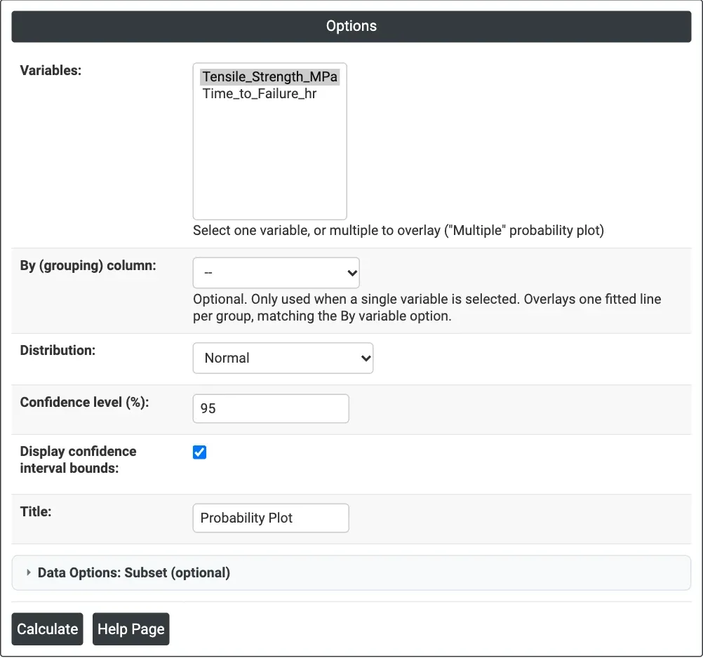
Figure 1 — Options for the example: Tensile_Strength_MPa on a Normal probability plot with 95% bounds.
Output Descriptions
- Probability Plot — the data (horizontal axis) against percent on the distribution's probability scale, with the fitted line and the dotted confidence bounds. The legend gives each series' AD statistic and its p-value.
- PDF export via Download.
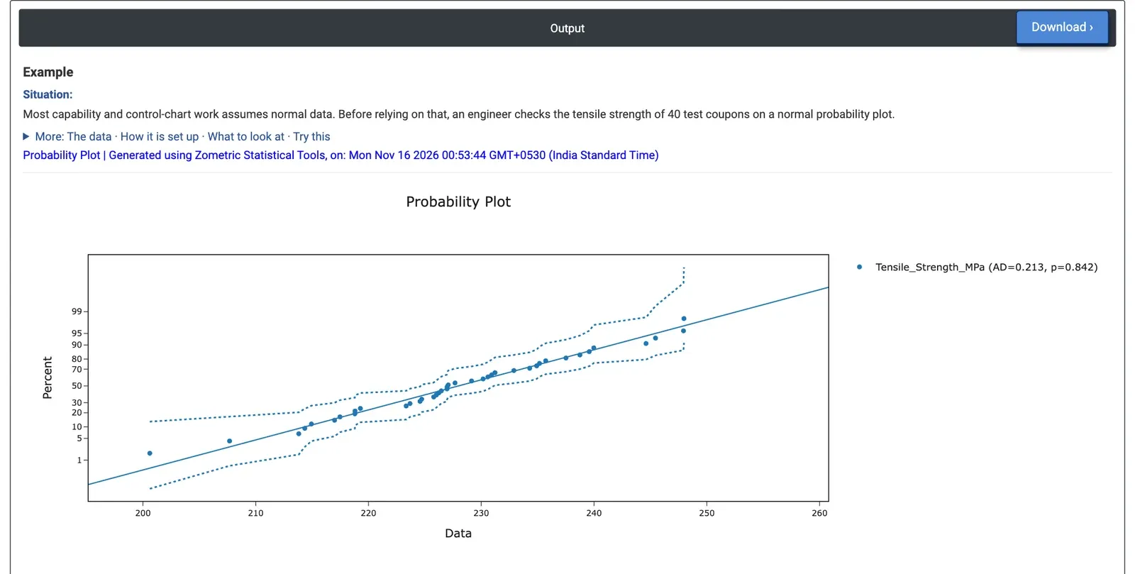
Figure 2 — Normal probability plot of the tensile strength of 40 coupons: AD = 0.213, p = 0.842.
Worked Example
Before setting control limits and calculating capability, an engineer checks whether the tensile strength of 40 test coupons can be treated as normal. Variables = Tensile_Strength_MPa, Distribution = Normal, Confidence level 95, bounds displayed.
The points follow the straight line and stay inside the dotted bounds over the whole range, from 200.61 to 247.97 MPa. The legend shows AD = 0.213 with p = 0.842, far above 0.05: there is no evidence against normality. The fitted line has mean 227.97 MPa and standard deviation 10.61 MPa, so normal-based capability and control-chart methods can be used. Points bending away from the line at either end would have pointed to a skewed or heavy-tailed distribution.
The same worksheet holds 40 times to failure (hours). Plotting Time_to_Failure_hr against several distributions gives AD = 0.210 with p > 0.250 for the Weibull (shape 3.23, scale 192.96 hours), AD = 0.158 with p = 0.947 for the Normal, AD = 1.228 with p < 0.005 for the Lognormal and AD = 7.628 with p < 0.010 for the Exponential. The Exponential, which assumes a constant failure rate, clearly does not fit, and neither does the Lognormal. The Weibull and Normal both fit well; for failure times the Weibull is the usual choice, since its shape above 1 describes wear-out and it cannot predict negative lives.
Frequently asked questions
How do you interpret a probability plot?
If the points follow the fitted straight line and stay inside the confidence bounds, the distribution fits. Points that leave the bounds are evidence against it, and points bending away from the line at either end suggest a skewed or heavy-tailed distribution. The legend gives the Anderson-Darling statistic and p-value; a p-value below 0.05 is evidence the data do not follow the distribution.
When should you use a probability plot?
Use it to check normality before capability analysis, control limits, tolerance intervals or t-tests that assume normal data. It is also used to choose a distribution, such as Weibull, lognormal or exponential, for reliability or non-normal capability work. Each variable or group needs at least 3 values, and several variables or groups can be overlaid.
How do you compare distributions on a probability plot?
Plot the same data against several distributions and compare the Anderson-Darling statistics and p-values; a smaller AD and a larger p-value usually mean a closer fit. In a worked example on 40 failure times, the Weibull (p > 0.250) and Normal (p = 0.947) fit well, while the Lognormal and Exponential (p < 0.010) do not.
Which distributions can a probability plot test?
Nine: Normal, Lognormal, Weibull, Exponential, 2-Parameter Exponential, Smallest Extreme Value, Largest Extreme Value, Logistic and Loglogistic. The Lognormal, Weibull, Exponential and Loglogistic need positive values, and the Lognormal, Weibull and Loglogistic use a logarithmic data axis, as on standard probability paper.