
T Chart (Time Between Events)
The T Chart monitors rare events by charting the time between successive occurrences instead of counts per interval. It fits an Exponential (default) or Weibull distribution to the non-negative gaps; the centre line is the fitted median and limits are its 0.135th and 99.865th percentiles. Nelson's rules 1 to 4 flag special causes. Output is the chart, a fit summary and special-cause points.
Last reviewed
Key takeaway
A T chart is a control chart for rare events that plots the time between successive occurrences, with limits from a fitted Exponential or Weibull distribution, making it more sensitive than c or u charts.
On this page
Purpose
A T Chart monitors rare events by charting the TIME (or other continuous measure) between successive occurrences, instead of counting events per fixed interval the way a c-chart or u-chart does. When events are rare, most fixed-interval counts are zero and a c/u chart becomes insensitive — a T chart reacts directly to each new gap, making it far more sensitive to a genuine change in the underlying event rate.
Key Capabilities
- Charts non-negative time-between-events data directly, with a choice of underlying distribution (Exponential or Weibull) rather than assuming Normality.
- Full Nelson's-rules special-cause detection (4 configurable rules) applied to the fitted chart.
- Row inclusion/exclusion and a separate “estimate parameters from” subgroup selector, so control limits can be baselined on a stable historical period while later points are plotted for comparison.
- Configurable X-axis scale for labeling the time axis.
Statistical Methods
Time-between-events data for rare events is typically right-skewed and is not well modeled by a Normal distribution, so the T chart fits either an Exponential or a Weibull distribution to the time-between-events series by maximum likelihood (the default is Exponential, the standard model for a constant, memoryless failure/event rate).
The center line is the fitted distribution's median (its 50th percentile), and the control limits are its 0.135th and 99.865th percentiles: LCL = max(0, dist.ppf(0.00135)), UCL = dist.ppf(0.99865) — the same tail probabilities a ±3σ Normal control chart would enclose, applied instead to the fitted, non-Normal distribution's own quantile function, which is the statistically correct way to set limits on skewed data rather than a raw mean ± 3σ on the untransformed scale.
Nelson's rules (special-cause detection) are then evaluated against the fitted control limits exactly as on the app's other control charts, flagging points beyond the limits (Rule 1), runs on one side of center (Rule 2), sustained trends (Rule 3), and alternating patterns (Rule 4).
Input Fields & Options
Field | Description |
Time between events | Required. The column of non-negative time (or other continuous measure) between successive rare events, in chronological order. |
Fit distribution | Exponential (default) or Weibull — the distribution fitted to the time-between-events series. |
Check Rule 1–4 / K for Rule 1–4 | The four Nelson special-cause rules, each independently toggled (defaults K = 3, 9, 6, 14). |
X scale | Optional custom labeling for the time axis. |
Include or Exclude / Specify which rows / Row numbers | Controls which rows are plotted. |
Specify subgroups to estimate parameters / Subgroups | Optionally restricts which rows are used to fit the distribution and set control limits, while still plotting all rows — useful for baselining on a known-stable period. |
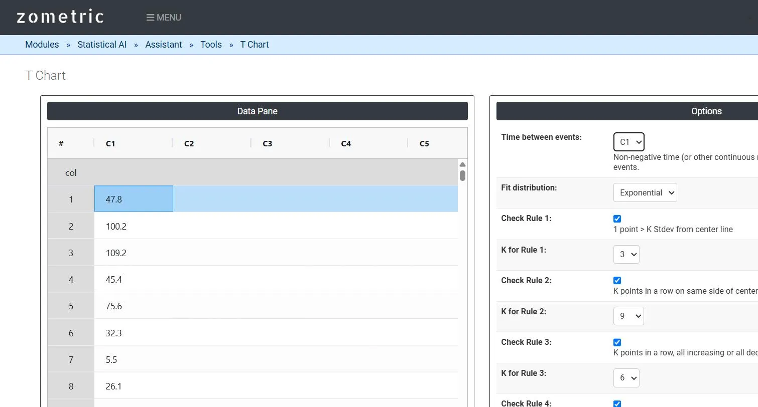
Figure 1 — 25 time-between-failure gaps (hours) pasted into C1, with Time between events set to C1 and Fit distribution = Exponential.
Output Descriptions
- T Chart plot — the time-between-events series in chronological order with UCL, center line and LCL from the fitted distribution.
- Fit summary table — the distribution fitted, center line, LCL and UCL.
- Nelson's Rules / Potential Special Cause Points — which rules were checked and which points (if any) violated them.
- PDF export via Download as PDF.
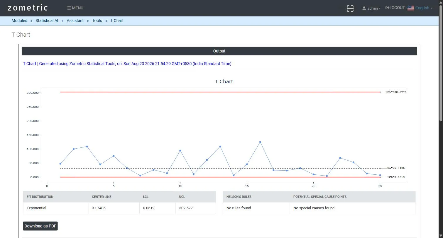
Figure 2 — T Chart output: fitted control limits, the plotted time-between-events series, and the fit-distribution/center-line/UCL/LCL summary table.
Worked Example
A plant tracks safety-relevant equipment failures on a packaging line, logging the number of hours between successive failures (25 successive gaps, column C1). With Fit distribution = Exponential, the tool fits an Exponential model to the gaps (Center Line ≈ 31.7, UCL ≈ 302.6, LCL ≈ 0.06) and plots all 25 gaps — giving an immediate visual read on whether the failure rate is accelerating (successive gaps shrinking toward the lower control limit) well before enough failures would accumulate to react on a traditional count-based chart.
Frequently asked questions
When should you use a T chart instead of a c chart or u chart?
Use a T chart when events are rare. With rare events most fixed-interval counts are zero, so a c or u chart becomes insensitive. A T chart charts the time between successive events and reacts directly to each new gap, making it more sensitive to a genuine change in the underlying event rate.
How are T chart control limits calculated?
An Exponential or Weibull distribution is fitted to the time-between-events data by maximum likelihood. The centre line is the fitted median, and the control limits are the 0.135th and 99.865th percentiles of that distribution, the same tail probabilities a plus or minus 3 sigma normal chart encloses, with the lower limit not below zero.
Why does the T chart not assume a normal distribution?
Time-between-events data for rare events are typically right-skewed and are not well modelled by a normal distribution. Setting limits from the fitted distribution's own quantiles is more appropriate for skewed data than a mean plus or minus 3 sigma on the untransformed scale. Exponential is the default, as the standard model for a constant event rate.
How do you interpret a T chart?
Points are the gaps between successive events in time order. Gaps shrinking towards the lower control limit suggest the event rate is increasing, such as failures accelerating. Nelson's rules flag points beyond the limits, runs on one side of the centre line, sustained trends and alternating patterns as potential special causes.